Transcription
Chapter 14Spline CurvesA spline curve is a mathematical representation for which it is easy to buildan interface that will allow a user to design and control the shape of complexcurves and surfaces. The general approach is that the user enters a sequenceof points, and a curve is constructed whose shape closely follows this sequence.The points are called control points. A curve that actually passes through eachcontrol point is called an interpolating curve; a curve that passes near to thecontrol points but not necessarily through them is called an approximating curve.the points are calledcontrol pointsinterpolating curveapproximating curveOnce we establish this interface, then to change the shape of the curve we justmove the control points.The easiest example to help us to understand how thisworks is to examine a curve that is like the graph of afunction, like y x2 . This is a special case of a polynomial function.y21-101x87
88CHAPTER 14. SPLINE CURVES14.1Polynomial curvesPolynomials have the general form:y a bx cx2 dx3 . . .The degree of a polynomial corresponds with the highest coefficient that is nonzero. For example if c is non-zero but coefficients d and higher are all zero,the polynomial is of degree 2. The shapes that polynomials can make are asfollows:degree 0: Constant, only a is non-zero.4.843.2Example: y 32.41.60.8-3-2.5-2-1.5-1-0.500.511.522.53-0.8A constant, uniquely defined by one point.degree 1: Linear, b is highest non-zero coefficient.4.843.2Example: y 1 2x2.41.60.8-3-2.5-2-1.5-1-0.500.511.522.53-0.8A line, uniquely defined by two points.degree 2: Quadratic, c is highest non-zero coefficient.4.843.2Example: y 1 2x x22.41.60.8-3-2.5-2-1.5-1-0.500.511.522.53-0.8A parabola, uniquely defined by three points.degree 3: Cubic, d is highest non-zero coefficient.1.60.8-3Example: y 1 7/2x -4A cubic curve (which can have an inflection, at x 0 in this example),uniquely defined by four points.The degree three polynomial – known as a cubic polynomial – is the one thatis most typically chosen for constructing smooth curves in computer graphics.It is used because1. it is the lowest degree polynomial that can support an inflection – so wecan make interesting curves, and2. it is very well behaved numerically – that means that the curves willusually be smooth like this:and not jumpy like this:.
14.1. POLYNOMIAL CURVES89So, now we can write a program that constructs cubic curves. The user entersfour control points, and the program solves for the four coefficients a, b, c and dwhich cause the polynomial to pass through the four control points. Below, wework through a specific example.Typically the interface would allow the user to entercontrol points by clicking them in with the mouse.For example, say the user has entered control points( 1, 2), (0, 0), (1, 2), (2, 0) as indicated by the dots inthe figure to the left.Then, the computer solves for the coefficients a, b, c, d and might draw the curveshown going through the control points, using a loop something like this:glBegin(GL LINE STRIP);for(x -3; x 3; x 0.25)glVertex2f(x, a b * x c * x * x d * x * x * x);glEnd();Note that the computer is not really drawing the curve. Actually, all it is doingis drawing straight line segments through a sampling of points that lie on thecurve. If the sampling is fine enough, the curve will appear to the user as acontinuous smooth curve.The solution for a, b, c, d is obtained by simultaneously solving the 4 linearequations below, that are obtained by the constraint that the curve must passthrough the 4 points:general form: a bx cx2 dx3 ypoint ( 1, 2): a b c d 2point (0, 0): a 0point (1, 2): a b c d 2point (2, 0): a 2b 4c 8d 0This can be written in matrix formM a y,
90CHAPTER 14. SPLINE CURVESor (one row for each equation) 1 1 11 1012 a21 1 b 0 0 0 1 1 c 2 d04 8The solution isa M 1 y,which is hard to do on paper but easy to do on the computer using matrix andvector routines.For example, using the code I have provided, you could write:Vector a(4), y(4);Matrix M(4, 4);y[0] 2; y[1] 0; y[2] -2; y[3] 0;// fill in all rows of MM[0][0] 1; M[0][1] -1; M[0][2] 1; M[0][3] -1;// etc. to fill all 4 rowsa M.inv() * y;After this computation, a[0] contains the value of a, a[1] of b, a[2] of c anda[3] of d. For this example the correct values are a 0, b 2 32 , c 0, andd 23 .14.2Piecewise polynomial curvesIn the previous section, we saw how four control points can define a cubicpolynomial curve, allowing the solution of four linear equations for the fourcoefficients of the curve. Here we will see how more complex curves can bemade using two new ideas:1. construction of piecewise polynomial curves,2. parameterization of the curve.Suppose we wanted to make the curve shown to the right.We know that a single cubic curve can only have one inflection point, but this curve has three, marked withO’s. We could make this curve by entering extra controlpoints and using a 5th degree polynomial, with six coefficients, but polynomials with degree higher than threetend to be very sensitive to the positions of the controlpoints and thus do not always make smooth shapes.
14.2. PIECEWISE POLYNOMIAL CURVES91The usual solution to this problem in computer graphics and computer aideddesign is to construct a complex curve, with a high number of inflection points,by piecing together several cubic curves: Here is one way that this can be done. Let each pair of control points representone segment of the curve. Each curve segment is a cubic polynomial with itsown 3x4x5x6x7x8xx9In this example, the ten control points have ascending values for the x coordinate, and are numbered with indices 0 through 9. Between each control pointpair is a function, which is numbered identically to the index of its leftmostpoint. In general, fi (x) ai bi x ci x2 di x3 is the function representing thecurve between control points i and i 1.Because each curve segment is represented by a cubic polynomial function, wehave to solve for four coefficients for each segment. In this example we have4 9 36 coefficients to solve for. How shall we do this?
92CHAPTER 14. SPLINE CURVESHere is one way:1. We require that each curve segment pass through its control points. Thus,fi (xi ) yi , and fi (xi 1 ) yi 1 . This enforces C 0 continuity – that is,where the curves join they meet each other.Note that for each curve segment this gives us two linear equations: ai bi xi ci x2i di x3i yi , and ai bi xi 1 ci x2i 1 di x3i 1 yi 1 . But tosolve for all four coefficients we need two more equations for each segment.2. We require that the curve segments have the same slope where they join0together. Thus, fi0 (xi 1 ) fi 1(xi 1 ). This enforces C 1 continuity –that is that slopes match where the curves join.Note that: fi (x) ai bi x ci x2 di x3 , so that fi0 (x) bi 2ci x 3di x2 .And C 1 continuity gives us one more linear equation for each segmentbi 2ci xi 1 3di x2i 1 bi 1 2ci 1 xi 1 3di 1 x2i 1 or bi 2ci xi 1 3di x2i 1 bi 1 2ci 1 xi 1 3di 1 x2i 1 0.3. To get the fourth equation we require that the curve segments have the00same curvature where they join together. Thus, fi00 (xi 1 ) fi 1(xi 1 ).This enforces C 2 continuity – that curvatures match at the join.Now: f 00 i(x) 2ci 6di xAnd C 2 continuity gives us the additional linear equation that we need2ci 6di xi 1 2ci 1 6di 1 xi 1 or 2ci 6di xi 1 2ci 1 6di 1 xi 1 04. Now we are almost done, but you should note that at the left end of thecurve we are missing the C 1 and C 2 equations since there is no segmenton the left. So, we are missing two equations needed to solve the entiresystem. We can get these by having the user supply the slopes at the twoends. Let us call these slopes s0 and sn .0This gives f00 (x0 ) s0 , and fn 1(xn ) sn so that b0 c0 x0 2d0 x20 s0 ,and bn 1 cn 1 xn 2dn 1 x2n sn .
14.2. PIECEWISE POLYNOMIAL CURVES93As we did with the case of a single cubic spline, we have a set of linear equationsto solve for a set of unknown coefficients. Once we have the coefficients we candraw the curve a segment at a time. Again the equation to solve isM a y a M 1 y,where each row of the matrix M is taken from the left-hand side of the linearequations, the vector a is the set of coefficients to solve for, and the vector y isthe set of known right-hand values for each equation.Following is a worked example with three segments:Segment 0: f0 (x)Slope at 0:Curve through (0, 1):Curve through (2, 2):Slopes match at join with f1 :Curvatures match at join with f1 :b0 2a0 1a0 2b0 4c0 8d0 2b0 4c0 12d0 b1 4c1 12d1 02c0 12d0 2c1 12d1 0Segment 1: f1 (x)Curve through (2, 2):Curve through (5, 0):Slopes match at join with f2 :Curvatures match at join with f2 :a1 2b1 4c1 8d1 2a1 5b1 25c1 125d1 0b1 10c1 75d1 b2 10c2 75d2 02c1 30d1 2c2 30d2 0Segment 2: f2 (x)Curve through (5, 0):Curve through (8, 0):Slope at 8:a2 5b2 25c2 125d2 0a2 8b2 64c2 512d2 0b2 16c2 192d2 1M a y, or
94 CHAPTER 14. SPLINE CURVES0110000000001021000000000000484 122 1200000000000000000001100000 a0000 0000 000 0000 b0 000 0000 c0 1 4 12 0000 d0 0 2 12 0000 a1 248 0000 b1 c1 5 25 125 0000 1 1075 0 1 10 75 d1 a2 0230 00 2 30 000 1525 125 b2 000 1864 512 c2 d2000 018 128212002000001 , soa M 1 y,Again, this is hard to solve by hand but easy on the computer.14.3Curve parameterizationSo far we have learned how a sequence of control points can define a piecewisepolynomial curve, using cubic functions to define curve segments between control points and enforcing various levels of continuity where segments join. Inparticular, we employed C 0 continuity, meaning that the two segments match values at the join. C 1 continuity, meaning that they match slopes at the join. C 2 continuity, meaning that they match curvatures at the join.We were able to determine coefficients for the curve segments via a set of linearequationsM a y a M 1 y,where a is the vector of all coefficients, y is the vector of constants on theright-hand side of the linear equations, and M is a matrix encoding the C 0 , C 1and C 2 conditions.This approach can be modified to specify each curve segment in parametricform, as indicated in the figure below.
14.3. CURVE PARAMETERIZATION95In the example, both curves are identical, however, the equations describingthem will be different. In the parametric form on the right, we have definedparameters t0 , t1 and t2 that vary between 0 and 1 as we step along the x axisbetween control points. We could write equations:t0t1t2dt0 1/2dxdt1 (x 2)/3, with 1/3dxdt2 (x 5)/3, with 1/3dx x/2,withrelating the t’s to the original x coordinate. The derivatives indicate how quicklyeach t varies as we move in the x direction.Now we specify each curve segment by a parametric cubic curvefi (ti ) ai bi ti ci t2i di t3iAt the left side of segment i, ti 0 and at the right ti 1, so C 0 continuity issimplyfi (0) ai yifi (1) ai bi ci di yi 1Notice, that in this form the ai coefficients are simply the y coordinates of theith control points, and do not have to be solved for.For C 1 continuity we differentiate once with respect to x using the chain rule:D x fi 0 fi dti1 fi, ti dxxi 1 xiand for C 2 continuity we differentiate twice:!000 fdtdti1iiDx2 fi fi. ti dx dx(xi 1 xi )2
96CHAPTER 14. SPLINE CURVESIt is important that these quantities be calculated in spatial (i.e. x), not inparametric coordinates, since we want the curves to join smoothly in space, notwith respect to our arbitrary parameterization.We force fi and fi 1 to match slopes by:(Dx fi )(1) (Dx fi 1 )(0),or(bi 2ci 3di )11 bi 1, or finallyxi 1 xixi 2 xi 1xi 1 xibi 1 0bi 2ci 3di xi 2 xi 1We force fi and fi 1 to match curvatures by:(Dx2 fi )(1) (D2 fi 1 )(0)or(2ci 6di )11 2ci 1, or finally2(xi 1 xi )(xi 2 xi 1 )2(xi 1 xi )22ci 6di 2ci 1 0.(xi 2 xi 1 )2Remember that we provided two extra equations by specifying slopes at the 2endpoints s0 and sn . So this gives00fn 1 (1)f0 (0) s0 , sn ,x1 x0xn xn 1orb0 (x1 x0 )s0 ,andbn 1 2cn 1 3dn 1 (xn xn 1 )sn .Looking back at our previous example, which we did without parameterization,we can rewrite all of our equations, and the final linear system that we have tosolve. On big advantage of this approach is that we reduce one row and onecolumn from the matrix for each control point, since we already know the valuesof all of the a coefficients.
14.4. SPACE CURVES97Segment 0: f0 (t0 )Slope at 0:Curve through (0, 1):Curve through (2, 2):Slopes match:Curvatures match:b0 (2 0)2 4a0 1a0 b0 c0 d0 2orb0 c0 d0 2 1 1b0 2c0 3d0 ( 2 05 2 )b1 02c0 6d0 2( 32 )2 c1 0Segment 1: f1 (t1 )Curve through (2, 2):Curve through (5, 0):Slopes match:Curvatures match:a1 2b1 c1 d1 0 2 2b1 2c1 3d1 ( 8 55 2 )b2 02c1 6d1 2c2 0Segment 2: f2 (t2 )Curve through (5, 0):Curve through (8, 0):Slope at 8:a2 0b2 c2 d2 0 0 0b2 2c2 3d2 (8 5)2 6M a y, or 11100000001220000001360000000 230110000 000 00 000 00 000 0 89 000 01 100 02 3 10 02 60 2 00 011 10 012 3 b0c0d0b1c1d1b2c2d2 4100 20006 , soa M 1 yOnce you have understood the notion of piecewise parameterization, the restfollows in a straightforward way.14.4Space curvesWe now know how to make arbitrary functions from a set of control points andpiecewise cubic curves, and we know how to use parameters to simplify theirconstruction. Now we will extend these ideas to arbitrary curves in two andthree dimensional space.
98CHAPTER 14. SPLINE CURVESFor the earlier examples, we used t for a parameter, but to distinguish the factthat we will now be looking at space curves, we will follow the usual notationin the literature and use the letter u.Suppose we have two functionsx u2 1,andy 2u2 u 3.As u varies, both x and y vary. We can make a table and we can plot the points.We see that the curve is described in 2-dimensional space, and unlike the graphof a function it can wrap back on itself. By picking appropriate functions x f (u) and y g(u) we can describe whatever 2D shape we desire.Suppose, for example, that we have a sequence of control points. Then betweeneach pair of points we can define two cubic curves as a function of a parameterthat varies from 0 to 1 between the control points and get a smooth curve
14.4. SPACE CURVES99between the points by applying C 0 , C 1 , C 2 constraints, as indicated by theexample in the following figure.In the figure, u1 is 0 at point 1 and 1 at point 2. A cubic curve is definedbetween points 1 and 2 byx ax1 bx1 u1 cx1 u21 dx1 u31 ,andy ay1 by1 u1 cy1 u21 dy1 u31 .We write two systems of linear equations for the x and y coordinates separately:Mx ax x and My ay y. Each system is solved following the same process weused in the previous sections; the only major difference being that we solve twolinear systems instead of one.Note that there are some differences in the details that have to be attended to.iFirst, instead of computing the single derivative dtdx for each segment as we did uiiabove, will now need the two derivatives x and u y for the chain rule. If welet each ui vary linearly from 0 to 1 for a segment between its control pointspi (xi , yi ) and pi 1 (xi 1 , yi 1 ) then ui1 , xxi 1 xiand1 ui . yyi 1 yiThere is one more point to consider. Now that wehave full space curves, it is quite possible for a curveto join back on itself to make a closed figure. If wehave this situation, and we enforce C 0 , C 1 and C 2continuity where the curves join, then we have all ofthe equations needed without requiring the user toenter any slopes.
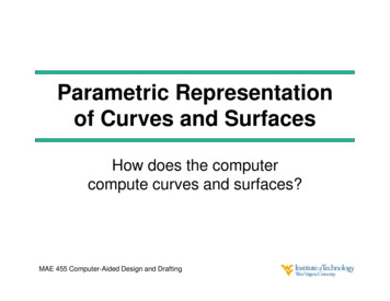
10014.5CHAPTER 14. SPLINE CURVESInterpolation methodsIn the notes we have worked through a method for building an interpolatingspline curve through a set of control points by using continuity C 0 , slope C 1and curvature C 2 constraints, where spline segments join. This is the method forcomputing natural cubic splines. It was very good for helping us to understandthe basic approach to constructing piecewise cubic splines, but it is not a verygood method for use in designing shapes. This is because the entire curve isdetermined by one set of linear equations M a y. Therefore, moving just onecontrol point will affect the shape of the entire curve. You can understand thatif you are designing a shape, you would like to be able to have local control overthe portion of the shape you are working on, without worry that changes youmake in one place may affect distant parts of the shape.For piecewise cubic interpolating curves, there are various ways of obtaininglocal shape control. The most important of these are Hermite Splines, CatmullRom Splines, and Cardinal Splines. These are explained quite well in a numberof computer graphics textbooks, but let us do a few examples to illustratethese methods. Note, for each example we will be looking at only one segmentof a piecewise curve. For each of these methods, each segment is calculatedseparately, so to get the entire curve the calculations must be repeated over allcontrol points.14.5.1Hermite cubic splinespi and pi 1 are two successive controlpoints. For Hermite Splines the user mustprovide a slope at each control point, in theform of a vector ti , tangent to the curve atcontrol point i. Letting parameter ui varyfrom 0 at pi to 1 at pi 1 , we use continuity C 0 and slope C 1 constraints at the twocontrol points.In the example to the left, pi (1, 1), and1 01ipi 1 (4, 3), thus dudx 4 1 3 , anddui1 01 . The tangent vectors aredy 3 1 2 01ti , and ti 1 .1.5 1The tangent vectors t are input by the user as direction vectors of the form
14.5. INTERPOLATION METHODS101 4x, but we need slopes in parametric form, so we compute the scaled4ytangents i4x du00dx ,Dpi 3i4y du( 23 )( 12 )dy4and"Dpi 1 i 14x dudxdui 14y dy# (1)( 31 )( 1)( 12 )Linear system for example Hermite SplineCurve passes through pi at ui 0:Curve passes through pi 1 at ui 1:Slope at pi :Slope at pi 1 :Thus in matrix form: 1 1 0001110102 ax0 bx1 0 cx3dx 1ay 4by cy 01dy3 13 12 .x(0) ax 1y(0) ay 1x(1) ax bx cx dx 4y(1) ay by cy dy 3x0 (0) bx 0y 0 (0) by 43x0 (1) bx 2cx 3dx 31y 0 (1) by 2cy 3dy 21 13 3 4 21Note, that the two matrices on the left-hand side of this equation are constant,and do not depend upon the control points or slopes. Only the matrix on theright varies with the configuration.14.5.2Catmul-Rom splinesIn the case of Catmul-Rom splines, pi andpi 1 are again two successive control points.Now, instead of requiring the user to enter slopes at each control point, we usethe previous point pi 1 and the subsequentpoint pi 2 to determine slopes at pi andpi 1 . The vector between pi 1 and pi 1is used to give the slope at pi and the vector between pi and pi 2 to give the slopeat pi 1 . We set ti 21 (pi 1 pi 1 ) andti 1 12 (pi 2 pi ).
102CHAPTER 14. SPLINE CURVESIn the example to the left, as in the previous example, pi (1, 1), and pi 1 dui11i(4, 3), thus again dudx 3 , and dy 2 .In addition, we have pi 1 (1, 1) andpi 2 (5, 2). Thus, the tangent vec tors are ti 21 (pi 1 pi 1 ) 2ti 1 12 (pi 2 pi ) . 32322, and 4xAgain, the tangent vectors t are in the form, but we need slopes in4yparametric form, so we compute the scaled tangents 3 1 1 i4x du( 2 )( 3 )dxDpi 2 ,i4y du1(2)( 12 )dyand"Dpi 1 i 14x dudxdui 14y dy# (2)( 31 )( 32 )( 12 ) Linear system for example Catmul-Rom SplineCurve passes through pi at ui 0:Curve passes through pi 1 at ui 1:Slope at pi :Slope at pi 1 :Thus in matrix form: 1 1 0014.5.301110102 0ax bx1 0 cx3dx 1ay 4by cy 122dy323 34 .x(0) ax 1y(0) ay 1x(1) ax bx cx dx 4y(1) ay by cy dy 3x0 (0) bx 21y 0 (0) by 1x0 (1) bx 2cx 3dx 23y 0 (1) by 2cy 3dy 34 13 1 43Cardinal splinesCardinal splines generalize the Catmul-Rom splines by providing a shape parameter t. With t 0 we have Catmul-Rom. Values of t 0 tighten the curve,making curvatures higher at the joins and values of t 0 loosen the curve. For
14.5. INTERPOLATION METHODSCardinal Splines:ti 1(1 t)(pi 1 pi 1 ),2andti 1 1(1 t)(pi 2 pi ).2103
92 CHAPTER 14. SPLINE CURVES Here is one way: 1. We require that each curve segment pass through its control points. Thus, f i(x i) y i, and f i(x i 1) y i 1.This enforces C0 continuity { that is, where the curves join they meet each other.