Transcription
InSight: RIVIER ACADEMIC JOURNAL, VOLUME 9, NUMBER 2, FALL 2013A STUDY OF CUBIC SPLINE INTERPOLATIONKai Wang ‘14G*Graduate Student, M.S. Program in Computer Science, Rivier UniversityAbstractThe paper is an overview of the theory of interpolation and its applications in numerical analysis. Itspecially focuses on cubic splines interpolation with simulations in Matlab .1 Introduction: Interpolation in Numerical MethodsNumerical data is usually difficult to analyze. For example, numerous data is obtained in the study ofchemical reactions, and any function which would effectively correlate the data would be difficult tofind. To this end, the idea of the interpolation was developed.In the mathematical field of numerical analysis, interpolation is a method of constructing new datapoints within the range of a discrete set of known data points (see below). Interpolation provides ameans of estimating of the value at the new data points within the range of parameters.What is the value y when t 1.25?2 Types of InterpolationsThere are several different interpolation methods based on the accuracy, how expensive is the algorithmof implementation, smoothness of interpolation function, etc.2.1 Piecewise constant interpolationThis is the simplest interpolation, which allows allocating the nearest value and assigning it to theestimating point. This method may be used in the higher dimensional multivariate interpolation, becauseof its calculation speed and simplicity.2.2 Linear interpolationLinear interpolation takes two data points, say (xa,ya) and (xb,yb), and the interpolation function at thepoint (x, y) is given by the following formula:x xay ya ( yb ya )xb xaLinear interpolation is quick and easy, but not very precise. Below is the error estimate formula,where the error is proportional to the square of the distance between the data points.Copyright 2013 by Kai Wang. Published by Rivier University, with permission.ISSN 1559-9388 (online version), ISSN 1559-9396 (CD-ROM version).1
Kai Wang1f ( x) g ( x) C ( xb x a )2 , where C max g ( y ) , y xa , xb .8Here g (x) is the interpolating function, which is twice continuously differentiable.2.3 Polynomial interpolationPolynomial interpolation is a generalization of linear interpolation. It replaces the interpolating functionwith a polynomial of higher degree.If we have n data points, there is exactly one polynomial of degree at most n 1 going through allthe data points:The interpolation error is proportional to the distance between the data points to the power n.f ( x) g ( x) ( x x1 )( x x2 ).( x xn ) ( n )f (c) , where c lies in x1 , xn .n!The interpolant is a polynomial and thus infinitely differentiable. With higher degree polynomial (n 1), the interpolation error can be very small. So, we see that polynomial interpolation overcomes mostof the problems of linear interpolation. However, polynomial interpolation also has some disadvantages.For example, calculating the interpolating polynomial is computationally expensive compared to linearinterpolation.Polynomial interpolation may exhibit oscillatory artifacts, especially at the end points (known asRunge's phenomenon). More generally, the shape of the resulting curve, especially for very high or lowvalues of the independent variable, may be contrary to common sense. These disadvantages can bereduced by using spline interpolation or Chebyshev polynomials [1-3].2.4 Spline interpolationSpline interpolation is an alternative approach to data interpolation. Compare to polynomialinterpolation using on single formula to correlate all the data points, spline interpolation uses severalformulas; each formula is a low degree polynomial to pass through all the data points. These resultingfunctions are called splines.Spline interpolation is preferred over polynomial interpolation because the interpolation error canbe made small even when using low degree polynomials for the spline. Spline interpolation avoids theproblem of Runge's phenomenon, which occurs when the interpolating uses high degree polynomials.The mathematical model for spline interpolation can be described as following:For i 1, ,n data points, interpolate between all the pairs of knots (xi-1, yi-1) and (xi, yi) withpolynomialsy qi(x), i 1, 2, ,n.The curvature of a function y f(x) is2
A STUDY OF CUBIC SPLINE INTERPOLATIONk y 3(1 y 2 ) 2As the spline will take a function (shape) more smoothly (minimizing the bending), both y and y should be continuous everywhere and at the knots. Therefore:qi ( xi ) qi 1 ( xi 1 ) and qi ( xi ) qi 1 ( xi 1 ) for i, where 1 i n 1This can only be achieved if polynomials of degree 3 or higher are used. The classical approachuses polynomials of degree 3, which is the case of cubic splines.3 Cubic Spline InterpolationThe goal of cubic spline interpolation is to get an interpolation formula that is continuous in both thefirst and second derivatives, both within the intervals and at the interpolating nodes. This will give us asmoother interpolating function. The continuity of first derivative means that the graph y S(x) will nothave sharp corners. The continuity of second derivative means that the radius of curvature is defined ateach point.3.1 DefinitionGiven the n data points (x1,y1), ,(xn,yn), where xi are distinct and in increasing order. A cubic splineS(x) through the data points (x1,y1), ,(xn,yn) is a set of cubic polynomials:S1 ( x) y1 b1 ( x x1 ) c1 ( x x1 ) 2 d1 ( x x1 ) 3 on[ x1 , x2 ]S2 ( x) y2 b2 ( x x2 ) c2 ( x x2 )2 d2 ( x x2 )3 on[ x2 , x3 ]Sn 1 ( x) yn 1 bn 1 ( x xn 1 ) cn 1 ( x xn 1 )2 dn 1 ( x xn 1 )3 on[ xn 1, xn ]With the following conditions (known as properties):a. Si ( xi ) yi and Si ( xi 1 ) yi 1 for i 1, ,n-1This property guarantees that the spline S(x) interpolates the data points.b. Si 1 ( xi ) Si ( xi ) for i 2, ,n-1S (x) is continuous on the interval x1 , xn ; this property forces the slopes of neighboring parts toagree when they meet.c. Si 1 ( xi ) Si ( xi ) for i 2, ,n-13
Kai WangS (x) is continuous on the interval x1 , xn , which also forces the neighboring spline to have thesame curvature, to guarantee the smoothness.3.2 Construction of cubic splineHow to determine the unknown coefficients bi, ci, di of the cubic spline S(x) so that we can construct it?Given S(x) is cubic spline that has all the properties as in the definition section 3.1,Si ( x) yi bi ( x xi ) ci ( x xi )2 di ( x xi )3 on[ xi , xi 1 ](1)for i 1, 2, ,n-1The first and second derivatives:Si ( x) 3di ( x xi )2 2ci ( x xi ) bi(2)Si ( x) 6di ( x xi ) 2ci(3)for i 1, 2, ,n-1From the first property of cubic spline, S(x) will interpolate all the data points, and we can haveSi ( xi ) yi .Since the curve S(x) must be continuous across its entire interval, it can be concluded that each subfunction must join at the data pointsSi ( xi ) Si 1 ( xi )Therefore,yi Si 1 ( xi )Si 1 ( xi ) yi 1 bi 1 ( xi xi 1 ) ci 1 ( xi xi 1 )2 di 1 ( xi xi 1 )3(4)yi yi 1 bi 1 ( xi xi 1 ) ci 1 ( xi xi 1 )2 di 1 ( xi xi 1 )3for i 2,3, ,n-1.(5)Letting h xi xi 1 in Eq. (5), we have:yi yi 1 bi 1h ci 1h2 di 1h3for i 2,3, ,n-1(6)Also, with properties 2 of cubic spline, the derivatives must be equal at the data points, that is4
A STUDY OF CUBIC SPLINE INTERPOLATIONSi 1 ( xi ) Si ( xi )(7)By Eq. (2), Si ( xi ) bi , andSi 1 ( xi ) 3di 1 ( xi xi 1 ) 2 2ci 1 ( xi xi 1 ) bi 1(8)bi 3di 1 ( xi xi 1 )2 2ci 1 ( xi xi 1 ) bi 1(9)Therefore,Again, letting h xi xi 1 , we find:bi 3di 1h2 2ci 1h bi 1for i 2,3, ,n-1(10)From Eq. (3), Si ( x) 6di ( x xi ) 2ci , we haveSi ( xi ) 6di ( xi xi ) 2ciSi ( xi ) 2ci(11)Since Si (x) should be continuous across the interval, therefore Si 1 ( xi ) Si ( xi )Si 1 ( xi ) 6di 1 ( xi xi 1 ) 2ci 1(12)2ci 6di 1 ( xi xi 1 ) 2ci 1Letting h xi xi 1 ,2ci 6di 1 ( xi xi 1 ) 2ci 12ci 6di 1h 2ci 1(13)Simplified these equation above by substituting DDi for Si ( xi ) , from Eq. (11)Si ( xi ) 2ci , DDi 2ciDDici 2(14)From Eq. (13):2ci 6di 1h 2ci 1 , 6di 1h 2ci 2ci 12c 2ci 1d i 1 i, substitute ci6hDDi DDi 1d i 1 ,6h5
Kai Wangor d i DDi 1 DDi6h(15)From Eq. (6):yi yi 1 bi 1h ci 1h2 di 1h3or yi 1 yi bi h ci h 2 di h3Therefore,yi 1 yi ci h 2 di h3 yi 1 yi bi (ci h d i h 2 )hhSubstitute ci and d iy y2 DDi DDi 1bi i 1 i h()h6(16)Put these systems into matrix form as follow:From Eq. (10),3di 1h 2 2ci 1h bi 1 bi .Substitute bi , ci d i :3(DDi DDi 1 2DDi 1y yi 12 DDi 1 DDiy y2 DDi DDi 1)h 2h i h() i 1 i h()6h2h6h6y 2 yi yi 1h( DDi 1 4 DDi DDi 1 ) i 16hDDi 1 4 DDi DDi 1 6(yi 1 2 yi yi 1)h2(17)for i 2, 3, , n-1Transform into the matrix equation: 1 0 0 0 0 0 4 101 410 14 0 00 0000 00 0 0 DD1 0 0 DD2 0 0 DD3 6 h2 0 0 DDn 1 1 0 DD n 4 1 y1 2 y2 y3 y 2y y 234 y3 2 y 4 y 5 yn 3 2 yn 2 yn 1 yn 2 2 yn 1 yn (18)6
A STUDY OF CUBIC SPLINE INTERPOLATIONThis system has n-2 rows and n columns, it is under-determined. In order to construct a unique cubicspline, two other conditions must be imposed upon the system.3.3 Cubic spline interpolation types3.3.1 Natural splineThere are several ways to add the two conditions. Let’s review the first scenario, Natural Spline.Natural-spline boundary conditions:S1 ( x1 ) 0 and Sn 1 ( xn ) 0(19)The Eq. (18) can be adapted accordingly to Eq. (20), because of DD1 0, DDn 0, 4 1 0 0 0 0 1 004 101 41 0 000 000 00 0 0 0 0 0 0 0 0 4 1 1 4 DD 2 DD3 6 2 h DDn 1 y1 2 y2 y3 y 2y y 234 y3 2 y 4 y 5 yn 3 2 yn 2 yn 1 yn 2 2 yn 1 yn (20)This is a diagonal linear system of the form HM V, which involves DD2, DD3, , DDn-1. Thislinear system in Eq. (20) is strictly diagonally dominant and has a unique solution. Then, using Eqs.(14), (15) and (16), coefficients ( bi , ci d i ) are determined. The cubic spline can be constructed.For example, data points (0,0), (1,0.5), (2, 1.8), (3,1.5), using the Matalab code for the solutionsabove, construct the unique cubic spline (namely, natural spline) for the data points (see Fig. 1).7
Kai WangFigure 1. The Natural Cubic Spline.3.3.2 Curvature-adjusted cubic splineThis type of spline is an alternative of natural spline, and sets S1 ( x1 ) and S n 1 ( xn ) to arbitrary value.This value corresponds to desired curvature settings at both end points.Boundary or Ending Points Conditions are: S1 ( x1 ) v1 and Sn 1 ( xn ) vn . The curvature-adjustedcubic spline is shown in Fig. 2 for the same data points (0,0), (1,0.5), (2, 1.8), (3,1.5), but with theconditions S1 ( x1 ) v1 1 , Sn 1 ( xn ) vn 1 .Figure 2. Curvature-Adjusted Cubic Spline.3.3.3 Clamped Cubic SplineThis type of spline is set end point first derivatives S1 ( x1 ) and S n ( xn ) to certain value, thus the slopeat the beginning and end of the spline are under user’s control.From Eq. (8) and Eq. (16), set S1 ( x1 ) v1,8
A STUDY OF CUBIC SPLINE INTERPOLATIONS1 ( x1 ) b1 y2 y12 DD1 DD2 h()h6We can have:6( y2 y1 ) 6hb1 h 2 DD22h 2Also from equation 8 and 16, set Sn 1 ( xn ) vn bn 1 ,DD1 (21)6( yn yn 1 ) 6hbn 1 2h 2 DDn 1(22)h2The clamped cubic spline is shown in Fig. 3 (below) for the same data points (0,0),(1,0.5), (2, 1.8),(3,1.5), and S1 ( x1 ) 0.5, Sn 1 ( xn ) 0.5.DDn Figure 3. Clamped Cubic Spline.3.3.4 Parabolically-Terminated Cubic SplineFor this type of spline, S1 ( x) and S n 1 ( x) are forced to be the functions of degree 2, which meansthat d1 d n 1 0.DDi 1 DDiFrom Eq. 15, d i , therefore:6hDD2 DD1 0, and DD1 DD2d1 6h1DDn DDn 1d n 1 0, and DDn DDn 16hn 1The parabolically-terminated cubic spline is shown in Fig. 4 (below) for the same data points(0,0),(1,0.5), (2, 1.8), (3,1.5).9
Kai WangFigure 4 Parabolically-Terminated Cubic Spline3.3.5 Not-a-Knot cubic splineTwo conditions d1 d 2 , d n 2 d n 1 were added to construct the unique spline. S1 ( x) and S 2 ( x)already agree at zeros, first and second derivatives. The condition d1 d 2 causes S1 ( x) and S 2 ( x) to beidentical cubic polynomials; thus the data-base point x2 is not needed anymore. Same thing is forSn 2 ( x) and S n 1 ( x) , and data point xn-1.DDi 1 DDiFrom Eq. (15), d i , therefore:6hDD3 DD2DD2 DD1, d2 , and d1 d 2 .d1 6h16h2Hence, DD1 DD2 h1 ( DD3 DD2 ).h2Also, d n 2 d n 1 ,DDn DDn 1DDn 1 DDn 2, d n 2 , and therefore:6hn 26hn 1h ( DDn 1 DDn 2 )DDn n 1 DDn 1hn 2d n 1 The not-a-knot cubic spline is shown below in Fig. 5 for data points (0,0), (1,0.5), (2, 1.8), (3,1.5), (4,0.8),and n 4.10
A STUDY OF CUBIC SPLINE INTERPOLATIONFigure 5. Not-a-Knot Cubic Spline.4. Cubic Spline Applications4.1 Representing functions by approximating polynomialsFirst, let’s review the application of a cubic spline to approximate polynomials, or to evaluate a cubicspline at certain point within the given interval [a, b].1As an example, consider the polynomial function f ( x) 2 sin( x) , on the interval [π/4, 3π/2]. Wexcan take few coupled data points: (π/4, 1.1463), (π/2, 0.4053), (3π/4, 0.1274), (π, 0), (5π/4, -0.0459),(3π/2, -0.0450). With natural cubic spline, the interpolating function is shown as a solid line in Fig. 6below. The exact values of the polynomial function f(x) (red markers) are also shown in Fig. 6.Comparing the results, we can see that the cubic-spline interpolating function approximates the exactfunction with a good accuracy.Figure 6. Comparing the Natural Cubic Spline Interpolating Function and the Exact Solution.11
Kai Wang4.2 Data correlation and interpolationData interpolation is widely used in real world, especially with large volume of irregular data. Findpolynomial functions guide these data within certain interval, can greatly help with data analysis anddata predicting. Cubic splines could be used for finding an interpolation function to correlate data.For example, in the chemical experiment, the following data was obtained (see arrays t and Dbelow and Fig. 7):t [0D [00.10.060 .499 0.50.17 0.190.60.211.00.261.40.291.50.291.899 1.90.30 0.312.0]0.31]We need to estimate the value D when t 1.2. Using the natural cubic spline interpolation (theformula Si ( x) yi bi ( x xi ) ci ( x xi )2 di ( x xi )3 on[ xi , xi 1 ] ), we found D 0.27527649.Figure 7. The Chemical Experiment Data, D f(t).ConclusionsIn this paper, we have presented an overview of the methods of interpolation and especially the cubicspline interpolation, which is widely used in numerous real-world applications. The study presents thedefinition of cubic spline interpolation and properties of different types of cubic splines, including anatural spline, a curvature-adjusted spline, a clamped spline, a parabolically-terminated spline, and a not-aknot spline. The spline construction formulas and corresponding Matlab codes were developed fordifferent types of cubic splines with excellent accuracy of calculation. Two general applications of cubicspline interpolation were also analyzed.References1.Interpolation. Wikipedia. Retrieved October 22, 2013, fromhttp://en.wikipedia.org/wiki/Interpolation12
A STUDY OF CUBIC SPLINE INTERPOLATION2.3.4.5.6.7.8.Spline Interpolation. Wikipedia. Retrieved October 22, 2013, fromhttp://en.wikipedia.org/wiki/Spline interpolationPolynomial Interpolation. Wikipedia. Retrieved October 22, 2013, fromhttp://en.wikipedia.org/wiki/Polynomial interpolationMathews, J. H., and Fink, K. K. Chapter 5: Curve Fitting. In: Numerical Methods Using Matlab,4th edition, Pearson, 2004.Introduction to Plotting with Matlab. Math Sciences Computing Center, University of Washington,September, 1996. Retrieved October 22, 2013, fromhttp://www.math.lsa.umich.edu/ tjacks/tutorial.pdfFriedman, J., Hastie, T., and Tibshirani, R. Chapter5: Splines and Applications. In: The Elements ofStatistical Learning. Retrieved October 22, 2013, fromhttp://www.cs.ubbcluj.ro/ csatol/mach learn/bemutato/BagyiIbolya SplinesAndApplications.pdfGrandine, T. A. The Extensive Use of Splines at Boeing. SIAM News, Vol. 38, No. 4, May 2005.Retrieved October 22, 2013, from http://www.me.ucsb.edu/ moehlis/ME17/splines.pdfCubic Spline Interpolation. Retrieved October 22, 2013, pline-interpolation.htmlApendix A: Matlab Code for the Project% Calculation of spline coefficients% Calculates coefficients of cubic spline% Input: x,y vectors of data points%plus two optional extra data v1, vn% Output: matrix of coefficients b1,c1,d1;b2,c2,d2;.function coeff Myproject(x,y,v1,vn)n length(x);A zeros(n-2,n-2);% matrix A is n-2xn-2r zeros(n-2,1);h zeros(n-1,1);for i 1:n-1h(i) x(i 1)-x(i);end% define the deltas% load the A matrixfor i 2:n-2A(i,i-1) 1;endfor i 1:n-2A(i,i) 4;endfor i 1:n-3A(i,i 1) 1;end%fprintf('display Matrix A\n');%disp(A);13
Kai Wangfor i 1:n-2r(i) 6*h(i)*(y(i)-2*y(i 1) y(i 2)); % right-hand sideendcoeff zeros(n-1,3);DD zeros(n,1);% natural spline conditionsv1 vn;%vn 0;%v1 0;% curvature-adj conditions%vn 0;%v1 0;MDD A\r;for i 2:n-1DD(i) MDD(i-1);end% natural spline conditions and curvature-adj conditionsDD(1) v1;DD(n) vn;%Clamped cubic spline%coeff(1,1) v1;%coeff(n,1) vn;%DD(1) (6*(y(2)-y(1))-6*h(1)*v1-h(1) 2*DD(2))/2*h(1) 2;%DD(n) (6*(y(n)-y(n-1))-6*h(n-1)*vn-2*h(n-1) 2*DD(n-1))/h(n-1) 2;% parabol-term conditions%DD(1) DD(2);%DD(n) DD(n-1);% not-a-knot%DD(1) DD(2)-(h(1)/h(2))*(DD(3)-DD(2));%DD(n) DD(n-1) (h(n-1)/h(n-2))*(DD(n-1)-DD(n-2));% solve for b, c d coefficientsfor i 1:n-1coeff(i,1) (y(i 1)-y(i))/h(i)-h(i)*(2*DD(i) DD(i 1))/6;coeff(i,2) DD(i)/2;coeff(i,3) (DD(i 1)-DD(i))/6;end14
A STUDY OF CUBIC SPLINE INTERPOLATION%calculate the certain value on interval [a,b], i 6%xd 1.2;%Dt y(6) coeff(6,1)*(xd-x(6)) coeff(6,2)*(xd-x(6)) 2 coeff(6,3)*(xd-x(6)) 3;%fprintf('%12.8f\n',xd,Dt);%plot the figure after calculation.clf;hold on;% clear figure window and turn hold onfor i 1:n-1x0 linspace(x(i),x(i 1),100);dx x0-x(i);y0 coeff(i,3)*dx;% evaluate using nested multiplicationy0 (y0 coeff(i,2)).*dx;y0 (y0 coeff(i,1)).*dx y(i);plot([x(i) x(i 1)],[y(i) y(i 1)],'o',x0,y0)end% plot the (1/x 2)*sin(x)%hold on%x1 pi/4:0.1:3*pi/2;%y1 x1. (-2).*sin(x1);%plot(x1, y1,'r*');hold offend* KAI WANG is a senior medical device and system product design engineer in Philips Healthcare Corp. He is a majorcontributor to several prime medical projects on software systems design, development, test and implementation in PhilipsHealthcare Corp. He completed Master Degree in Computer Science at Rivier University, Nashua, NH, in January2014. He also holds B.S. Degree from Harbin University of Science and Technology and M.S. Degree from TianJinUniversity.15
A STUDY OF CUBIC SPLINE INTERPOLATION 2 3 (1 y) y k c c As the spline will take a function (shape) more smoothly (minimizing the bending), both yc and yc should be continuous everywhere and at the knots. Therefore: q i (x i) q i c 1 (x i 1) and c( ) c 1 ( 1) q i x i q i x i for i, where 1did n 1 This can only be achieved if polynomials of .