WIXLIB

192.3: According to a report from the Newspaper Advertising Bureau, 40% of all primarycar maintainers are women. Consequently, advertisements for car care products,traditionally geared toward men, are now being aimed at women also. Consider thepopulation consisting of all primary car maintainers.a. What is the probability that a primary car maintainer, selected from thepopulation, is a woman? A man?b. What is the probability that both primary car maintainers in a sample of twoselected from the population are women?SolutionP(woman) .40P(man) .60b) What is the probability that both car maintainers in a sample of two selected from thepopulation are women?P(W) .40 * .40 .162.4: For two events A and B, P(A) .5, P(B) .6, and P(both A and B occur) .4. Findthe probability that either A or B or both occur.Solutiona) Are events A and B independent?P(A) .6, P(B) .4 and P(A B) .15. They are not independent, because P(A B) P(A)b) Are events A and C independent?P(A) .6, P(C) .5 and P(A C) .5. They are not independent, because P(A C) P(A)c) Are events B and C independent?P(B) .4, P(C) .5 and P(B C) .3. They are not independent, because P(B C) P(B)2.5: P(A or B or both) P(A) P(B) – P(A and B) .5 .6 - .4 .7The merging process from an acceleration lane to the through lane of a freewayconstitutes an important aspect of traffic operation at interchanges. From a study ofparallel and tapered interchange ramps in Israel, the table provides information on traffic19

20lags (where a lag is defined as an interval of time between arrivals of major streams ofvehicles) accepted and rejected by drivers in the merging lane.Type ofInterchangeLaneTaperedParallelTrafficConditionOn FreewwayHeavy TrafficLittle TrafficHeavy TrafficLittle TrafficNumber of MergingDrivers Acceptingthe First AvailableLag166740144Number of MergingDrivers Rejectingthe First AvailableLag115121139331a. What is the probability that a driver in a tapered merging lane with heavy trafficwill accept the first available lag?b. What is the probability that a driver in a parallel merging lane with heavy trafficwill reject the first available lag?c. Given that a driver accepts the first available lag in little traffic, what is theprobability that the driver is in a parallel merging lane?a)b)c)20

213. Probability Distributions with Applications3.1: A discrete random variable can assume 5 possible values, as listed in theaccompanying probability distribution.XP (x)1.202.254-5.308.10a. Find the missing value for p(4).b. Find the probability that x 2 or x 4.Solutiona) P (4) 1 – (.20 .25 .30 .10) .15b) x 2 or x 4?P(2) .25P(4) .15P(x 2 or x 4) P(2) P(4) .25 .15 .40c) P(x 4) P(1) P(2) P(4) .20 .25 .15 .603.2: Find µ and σ for the probability distribution in exercise 3.1Solution3.3: A coin is tossed 10 times and the number of heads is recorded. To a reasonabledegree of approximation, is this a binomial experiment? Check to determine whethereach of the five conditions required for a binomial experiment is satisfied.SolutionThe example is a binomial experiment, because it meets all the required conditions for abinomial experiment.1. A sample of n experiment units is selected from a population.Yes, n is 10 in this example.21

222. Each experimental unit possesses one of two characteristics, success or failure.Each flip of the coin is one experimental unit. Heads can represent “success”, while thetail represents “failure”.3. The probability that a single experimental unit possesses the “success” characteristic isequal to π. This probability is the same for all experimental units.Each flip of coin has the same probability of having a “success” or a “failure”.4. The outcome for any one experimental unit is independent of the outcome for anyother experimental unit.Each flip of coin is independent of the other.5. The random variable x counts the number of “successes” in n trails.This is also true for tossing of coins.3.4: In a study, Consumer Reports found widespread contamination and mislabeling ofseafood in the markets in New York City and Chicago. The study revealed one alarmingstatistic: 40% of the swordfish pieces available for sale had a high level of mercury abovethe Food and Drug administration (FDA) maximum amount. In a random sample of thethree swordfish pieces, find the probability that:a. All three swordfish pieces have a mercury level above FDA maximum.b. Exactly one swordfish piece has a mercury level above the FDA maximum.c. At most one swordfish piece has a mercury level above the FDA maximum.Solutiona)b)c) P(x 0 or x 1) P(x 0) P(x 1)22

23P(x 0 or x 1) .216 .432 .6483.5: Occupational Outlook Quarterly recently reported that 1% of all the drywallinstallers employed in the construction industry are women. In a random sample of 10drywall installers find the probability that at most one is a woman.SolutionA binomial distribution with n 10, and π 0.01P(at most one woman) P (x less than OR equal to 1)From the Binomial, with n 10 and π 0.01, we find P(at most one woman) 0.99573.6: According to the American Hotel and Motel Association, women are expected toaccount for half of all business travelers by the last year. To attract these women businesstravelers, hotels are providing more amenities that women particularly like, such asshampoo, conditioner, and body lotion. A survey of American hotels found that 86%offer shampoo in their guest rooms. Consider random sample of five hotels, and let x bethe number that provide shampoo as a guest room amenity.a. To a reasonable degree of approximation, is this a binomial experiment?b. What is the “success” in the context of this experiment?c. What is the value of π ?d. Find the probability that x 4.e. Find the probability that x 4.SolutionA). Yes, because:1. n 52. Two outcomes3. π 86%4. outcome independent5. random variable counts number of successesTherefore qualifies as a binomial experiment.B.) a hotel that has shampooC.) pie 86%D.) P(x 4) 0. 382923

24E.) P(x 4) P (4) P (5) 0.3829 0.4704 0.85333.7: Find the area under the standard normal curve:a. Between z 0 and z 1.96b. Between z -1.96 and z 0c. Between z -1.96 and z 1.96d. For values of z larger than .55f. For values of z less than –1.24.Show the values of z and corresponding area of interest on a sketch of the normal curvefor each part of the exercise.SolutionUsing the left margin column together with the top margin row of Normal Table:A.)B.)C.)D.)E.).4750.47500.4750 0.4750 .95000.5 - 0.2088 0.29120.5 - 0.3925 0.10753.8: Find the value of z (to 2 decimal places) that cuts off an area in the upper tail of thestandard normal curve equal to:a. 0.25b. 0.05c. 0.005d. 0.01e. 0.10Show the area and corresponding value of z on a sketch of the normal curve for each partof the exercise.SolutionLooking in the body of Normal TableA.)B.)C.)D.)E.)1.961.64 or 1.65. Better to say 1.6452.57 or 2.58. Better to say 2.5752.331.283.9: Find the approximate value for z0 such that the probability that z is larger than z0 is:24

25a. P .10b. P .15c. P .20d. P .25Locate z0 and the corresponding probability P on a sketch of the normal curve for eachpart of the exercise.SolutionP-value is the area to the tail, therefore using Normal Table:A.)B.)C.)D.)1.281.04.84.673.10: Researchers have developed sophisticated intrusion-detection algorithms to protecteth security of computer-based systems. These algorithms use principles of statistics toidentify unusual or expected data, i.e., “intruders.” One popular intrusion-detectionsystem assumes the data being monitored are normally distributed. As an example, theresearcher considered system data with a mean of .27, a standard deviation of 1.473, andan intrusion-detection algorithm that assumes normal data.a. Find the probability that a data value observed by the system will fall between - .5and .5.b. Find the probability that a data value observed bye the system exceeds 3.5.c. Comment on whether a data value of 4 observed by the system should beconsidered an “intruder”.SolutionAfter Z-transformation of the random variable X, you use Normal Table:A.)B.)C.)x between -0.5, and 0.5 is equivalent to z between -.53 and 0.16. UsingFrom Normal Table, we have 0.2019 0.0636 0.2655x greater than 3.5 is equivalent to z greater than 2.19. UsingFrom Normal Table, we have 0.5 - 0.4857 0.0143Based on Part B. an observed value of 4 is very unlikely, therefore, it isan “intruder”3.11: The Journal of Information Systems study of intrusion-detection systems.According to the study many intrusion-detection systems assume that data beingmonitored are normally distributed when such data are clearly non-normal. Consequently,the intrusion-detection system may lead to inappropriate conclusions. Te researcherconsidered the following data on input-output (I/O) units utilized by a sample of 44 usersof a system.25

0Based on the accompanying MINITAB printouts, assess whether the data are normallydistributed.Stem-and-leaf of I/OLeaf Unit 1.0(26)181411854421100000111112N 000Q10.000Q35.750STDEV5.160SEMEAN0.778SolutionThe stem and leaf plot does not show a symmetric shape3.12: Suppose x is a uniform random variable over the interval 1 x 3. Find thefollowing probabilities:a. P (x 2.5)b. P ( x 1.7)c. P (1.5 x 2)d. P ( x 2)e. p(1.1 x 1.6)f. P(x 1.3)26

27SolutionA.) P(X C) C-AB-AB.) P(X 1.7) P(X 2.5)3-1.73-1 2.5-13-1 1.5 .752 0.65C.) P(1.5 X 2) 0.25Similarly:D.) 0.5E.) 0.25F.) 0.15µ Mean a b2 2/5d 2d2σ S.D. b-aSquare root of 12 2.4d2 2d-2/5d3.46 1.2d.462dµ σ (0.74d, 1.66d)µ 2σ (0.28d, 2.12d)The height of the rectangle is 1/(b-a) 1/(2d -2d/5) 0.625dB.) P( x d) (c - a)/(b - a) (d -.4d) /(2d - .4d) .6d/1.6d 0.375.27

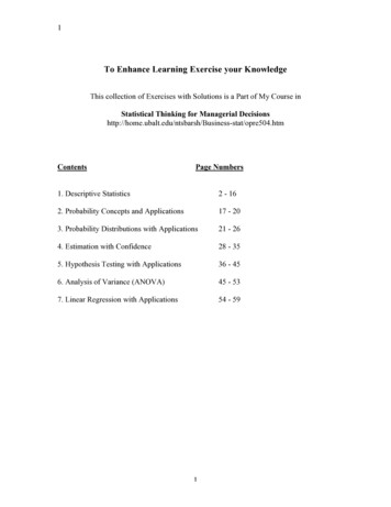
284. Estimation with Confidence4.1: Suppose a random sample of n measurements is selected from a population withmean µ 60 and variance σ ² 100. For each of the following values of n, give the meanand standard deviation of the sampling distribution of the sample mean, x:a. n 10b. n 25c. n 50d. n 75e. n 100f. n 500g. n 1,000Solutionµ 60,nMeanStandard 0600.4471000600.316For ex a)4.2: The National Institute for Occupational Safety and Health (NIOSH) recentlycompleted a study to evaluate the level of exposure of workers to the chemical dioxin, 2,3, 7, 8-TCDD. The distribution of TCDD levels in parts per trillion (ppt) in productionworkers at a Newark, New Jersey, chemical plant had a mean of 293 ppt and a standarddeviation of 847 ppt. A graph of the distribution is shown here.20.1050010001500200028

29In a random sample of n 50 workers selected at eth New Jersey plant, let x representthe sample TDCC level.a. Find the mean and standard deviation of the sampling distribution of x.b. Draw a sketch of the sampling distribution of x. Locate the mean on the graph.c. Find the probability that x exceeds 550 ppt.Solutionn 50, µ 293,a) µ 293,b)µ 293c) z-score P(x exceeds 550ppt) 0.5 – 0.4842 0.0158 1.58%4.3: The manufacturer of a new instant-picture camera claims that its product had “theworld’s fastest-developing color film by far.” Extensive laboratory testing has shown thatthe relative frequency distribution for the time it takes the new instant camera to begin toreveal the image after shooting has a mean of 9.8 seconds and a standard deviation of .55second. Suppose 50 of these cameras are randomly selected from the production line andtested. The time until the image is revealed, x, is recorded fro each.a. Describe the sampling distribution of x, the mean time it takes the sample of 50cameras begin to reveal the image.b. Find the probability that the mean time until the image is first revealed for the 50sampled cameras is greater than 9.70 seconds.c. If the mean and standard deviation of the population relative frequencydistribution for the times until the cameras begin to reveal the image are correct,would you expect to observe a value of x less than 9.55 seconds? Explain.29

30d. Refer to part a. Describe the changes in the sampling distribution of x if thesample size were decreased from n 50 to n 20.e. Repeat part d if the sample size were increased from n 50 to n 100.Solutionn 50, µ 9.8,a) It is approximately normal. The standard deviation of the sampling distribution wouldbe smaller than that of the population.b)z-score (9.7 – 9.8) / 0.07778 -1.286P(x 9.70) 0.5 0.4015 0.9015c) z-score (9.55 – 9.8) / 0.07778 -3.21P(x 9.55) 0.00065. The probability is almost zero. I would not expect to observe avalue less than 9.55 seconds.d) n 20 , with a smaller sample size, the sampling distribution would become morespread out and start to deviate from normale) n 100, with a larger sample size, the sampling distribution would become less spreadout and would be closer to normal distribution.4.4: A random sample of size n is selected from an unknown population with mean µ andstandard deviation σ. Calculate a 95% confidence interval for µ for each of eth followingsituations:a. n 35, x 26, s² 228.2b. n 70, x 24.1, s² 198.4c. n 105, x 24.2, s² 216.9Solution95% confidence 420.8027.4010524.2216.921.3827.0230

314.5: According to a study in Administrative Science Quarterly, the salary gap betweenChief executive officer (CEO) of a firm and a Vice President (VP) is often very large,and the gap appears to increase the more VPs a firm employs. Based on data collected fora sample of 105 U.S. firms drawn from Business Week’s executive CompensationScoreboard, the mean and standard deviation of the number of VPs employed by a firmare x 19.4 and s 10.1. Use this information to estimate the true mean number of VPsat U.S. firms with a 90% confidence interval. Interpret the result.Solutionnxbarsminmax10519.410.117.7821.02We are 90% confident that the mean number of VPs for all US firms will fall between 18and 21.4.6: Give two reasons why the CLT-based interval estimation procedure for thepopulation mean may not be applicable when the sample size is small.SolutionWhen the sample size is small, the central limit theorem does not apply. The standarddeviation of the sample does not approximate the true standard deviation of thepopulation.4.7: The following data represent a random sample of five measurements from anormally distributed population:742a. Find a 90% confidence interval for µ.57B. Find a 99% confidence interval for µ.31

32Solutiona) 90% confidence interval, t 2.132 (From the T-Table)b) 99% confidence interval, t 4.604 (From T-Table)4.8: Consider two independent random samples, 30 observations selected frompopulation 1 and 40 selected from population 2. The resulting sample means andvariances are shown in the table.a.b.c.Sample fromPopulation 1Sample fromPopulation 2x 1 15s² 1 16n1 30 x 2 23s²2 100n2 40Construct a 90% confidence interval for (µ1 - µ2 ).Construct a 95% confidence interval for (µ1 - µ2 ).Construct a 99% confidence interval for (µ1 - µ2 ).Solutiona) 90% confidence intervalb) 95% confidence intervalc) 99% confidence interval32

334.9: A Harris Corporation/University of Florida study was undertaken to determinewhether a manufacturing process performed at a remote location can be establishedlocally. Test devices (pilots) were set up at both the old and new locations, and voltagereadings on the process were obtained. A “good process” was considered to be one withvoltage readings of at least 9.2 volts (with larger readings being better than smallreadings).The table contains voltage readings for 30 production runs at each location.Descriptive statistics for both sample data sets are provided in the SAS printout below.We wish to determine whether a manufacturing process performed at a remote locationcan be established locally, test devices (pilots) were set up at both the old and newlocations and voltage readings on 30 production runs at each location were obtained. Thedata are reproduced in the table. Descriptive statistics are displayed in the accompanyingSAS printout. [Note: larger voltage readings are better tan smaller voltage 979.87Old .6310.109.7010.099.6010.0510.129.499.37New 8.828.658.519.149.758.789.359.549.368.68Analysis Variable: ATION OLD------------------------------------------N Obs NMinimumMaximumMeanStd ----------30 308.050000010.5500000 ----------------LOCATION NEW----------------------------------------N Obs NMinimumMaximumMeanStd ----30 308.510000010.1200000 9.42233330.478875733

34a. Compare the mean v

Descriptive Statistics 2 - 16 2. Probability Concepts and Applications 17 - 20 3. Probability Distributions with Applications 21 - 26 . The Empirical rule states that close to 95% of observations will lie in this range for symmetric distributions, it also states that the percentage will be near 100% for highly