WIXLIB

4Mathematical Problems in Engineeringimaging fMRI data from the human brain. We use this to illustrate the effect of the meanfield assumption implicit in DEM and establish the face validity of Generalised Filtering interms of known neurobiology. We conclude with a brief discussion.2. Generalised FilteringIn this section, we present the conceptual background and technical details behindGeneralised Filtering, which in principle can be applied to any nonlinear state-space ordynamic causal model formulated with stochastic differential equations. Given the simplicityof the ensuing scheme, we also take the opportunity to consider state-dependant changes inthe precision of random fluctuations. This represents a generalisation of our previous workon dynamic causal models and will be exploited in a neurobiological context, as a metaphorfor attention Feldman et al.; in preparation . However, we retain a focus on cascades of statespace models, which we have referred to previously as hierarchical dynamic models 13 .2.1. Filtering from Basic PrinciplesGiven a model m and generalised sensor data s s, s , s , . . . T Rp comprising real values,their velocity, acceleration, jerk, and so forth, we want to evaluate the log-evidence integratedover the time t 0, T that data are observed cf. 14, 15 :ε Tdt ln p s t m . 2.1 0Generally, this path-integral cannot be evaluated directly; however, one can induce an upperbound S ε that can be evaluated with a recognition density q t : q ϑ t on the causes i.e., states and parameters of the data. We will see later that these causes comprise timevarying states u t ϑ and slowly varying parameters ϕ t ϑ. This bound is based on freeenergy, which is constructed by simply adding a nonnegative term DKL t to the negative log-evidence 11, 16, 17 . The resulting integral is called free-action because it is a pathintegral of free-energy see also 18 S dtF t ε,F t ln p s t m DKL t , DKL t ln q ϑ t ln p ϑ t s t , m q . 2.2 By Gibb’s inequality the Kullback-Leibler divergence DKL t 0 is greater than zero, withequality when q t p ϑ t s t , m : t 0, T is the true conditional density. In this case, negative free-action becomes accumulated log-evidence S ε. Minimising this bound, byoptimising the recognition density at each time point, makes it an approximate conditionaldensity on the causes and makes free-action a bound approximation to the accumulated logevidence. The approximate conditional density can then be used for inference on the states orparameters of a particular model, and the accumulated log-evidence can be used to comparedifferent models e.g., 19 .

Mathematical Problems in Engineering5Crucially, the free-energy can be evaluated easily because it is a function of q ϑ t anda generative model p s t , ϑ t m entailed by mF t L t q H t ,L t ln p s t , ϑ t m , H t ln q t q . 2.3 The free-energy has been expressed here in terms of H t , the negentropy of q t , and anenergy L t expected under q t . In physics, L t is called Gibb’s energy and is a logprobability that reports the joint surprise about data and their causes. If we assume thatq ϑ t N μ t , C t is Gaussian the Laplace assumption , then we can express freeenergy in terms of its sufficient statistics, the mean and covariance of the recognition density F L μ 1n1 tr CLμμ ln C ln 2πe,222 2.4 where n dim μ . Here and throughout, subscripts denote derivatives. We can nowminimise free-action with respect to the conditional precisions P t C t 1 inversecovariances by solving δC S 0 C F 0 to giveFΣ 11Lμμ P 0 P Lμμ .22 2.5 Equation 2.5 shows that the precision is an analytic function of the mean, which meansall we have worry about is the approximate conditional mean. One can see this clearly byeliminating the conditional covariance to express the free-energy as a function of and onlyof the conditional means F L μ n1 ln Lμμ ln 2π.22 2.6 The conditional means, which minimise free-energy, are the solutions to the followingordinary differential equations. For the generalised states u t ϑ these equations are u μ Dμ u Fu μ̇ u μ u Fu μ̇ u μ u Fu μ̇ u μ u Fu . 2.7

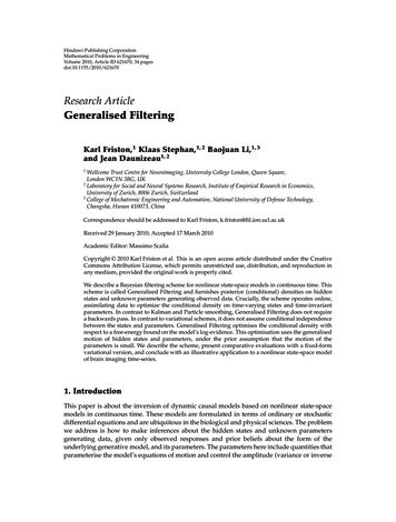
6Mathematical Problems in Engineeringwhere D is a derivative matrix operator with identity matrices above the leading diagonal,such that D u u , u , . . . T . Here and throughout, we assume that all gradients are evaluatedat the mean; here u t μ u t . The stationary solution of 2.7 , in a frame of reference thatmoves with the generalised motion of the mean, minimises free-energy and action. This canbe seen by noting that the variation of free-action with respect to the solution is zero: u u 0 Fu 0 δu S 0.μ Dμ 2.8 This ensures that when Gibb’s energy is minimized, the mean of the motion is the motion of u the mean, that is, Fu 0 μ Dμ u . For slowly varying parameters ϕ t ϑ this motiondisappears and we can use the following scheme:μ̇ ϕ μ ϕ ,μ̇ ϕ Fϕ κμ ϕ . 2.9 ϕ Here, the solution μ 0 minimises free-energy, under constraint that the motion of the ϕ mean is small; μ 0. This can be seen by notingμ̇ ϕ μ̇ ϕ 0 Fϕ 0 δϕ S 0. 2.10 Equations 2.7 and 2.9 prescribe recognition filtering dynamics for expected states andparameters respectively. The dynamics for states can be regarded as a gradient descent in aframe of reference that moves with the expected motion cf. a moving target . Conversely,the dynamics for the parameters can be thought of as a gradient descent that resists transientfluctuations in free-energy with a damping term κμ ϕ . This instantiates our prior belief thatfluctuations in the parameters are small, where κ can be regarded as a prior precision. Figure 1shows the implicit kernel solid line that is applied to fluctuating free-energy gradients toproduce changes in the conditional mean. It can be seen that the height of the kernel is 1/κ.We find that using κ 8T ensures stable convergence in most situations. This renders theintegral of the kernel over the time-series about one eighth see Appendix A for a discussionof this assimilation scheme in relation to classical methods .The solutions of 2.7 and 2.9 produce the time-dependent moments of anapproximate Gaussian conditional density on the unknown states and parameters. These canbe used for inference on states or parameters directly or for model comparison using the bound on accumulated log-evidence see 2.3 and 2.6 . Because the conditional meansof the parameters change slowly over time unlike their conditional precisions , we cansummarise the conditional estimates with the conditional density on the average over time ϕusing Bayesian parameter averaging ϕ ,q ϕ N μ ϕ , C ϕ μ ϕ C ϕ 1C P ϕ t μ ϕ t dt, P ϕ t dt. 2.11

Mathematical Problems in Engineering7Gradient accumulating kernels10.8Δμ ϕ t 0K s Lϕ t s ds0.6Δμ ϕ t 0K s Lϕ t s ds0.41KK t 0.2000.51Time s 1.52K t Figure 1: This graph shows the kernels implied by the recognition dynamics in 2.9 that accumulateevidence for changes in the conditional estimates of model parameters. These kernels are applied to thehistory of free-energy gradients to produce changes in the conditional mean solid line and its motion broken line . The kernels are derived from a standard Volterra-series expansion about the true conditionalmean, where, in this example, κ 4. ϕ Here, μ ϕ and C are the conditional moments of the average while μ ϕ t μ t andP ϕ t 1 C ϕ t C t are the mean and precision of the marginal conditional densityon the parameters at each point in time. This summary will be overconfident because itneglects conditional dependencies due to temporally correlated random terms and the useof generalised data . However, it usefully connects the conditional density with posteriordistributions estimated in conventional schemes that treat the parameters as static.In Generalised Filtering, changes in the conditional uncertainty about the parametersare modelled explicitly as part of a time-varying conditional density on states and parameters.In contrast, variational schemes optimise a conditional density on static parameters, that is,q ϕ that is not a functional of time although fluctuations in the conditional dependencebetween states and parameters are retained as mean-field terms that couple their respectivemarginals . This difference is related to a formal difference between the free-energy boundon log-evidence in variational schemes and free-action. Variational schemes return the freeenergy of the accumulated data e.g., see 3, equation 9 . Conversely, in GeneralisedFiltering, the free-energy is accumulated over time. This means that the variational freeenergy FV bounds the log-evidence of accumulated data, while free-action S dtF t bounds the accumulated log-evidence of data S dt ln p s t m , VF ln ps t m .t 2.12

8Mathematical Problems in EngineeringThese are not the same because evidence is a nonlinear function of the data see, Appendix Bfor an example . This distinction does not mean that one form of evidence accumulationis better than another; although it raises interesting issues for model comparison that willbe pursued elsewhere Li et al; in preparation . For the moment, we will approximate thefree-action associated with the conditional densities from variational schemes by assuming ϕ that q u t , ϕ q u t q ϕ , where q ϕ N μ ϕ , C ϕ and C ϕ T C Appendix B .This allows us to compare fixed-form schemes with DEM and without GF the mean fieldassumption, in terms of free-action.2.2. SummaryIn summary, we have derived recognition or filtering dynamics for expected states andparameters in generalised coordinates of motion , which cause data. The solutions to theseequations minimise free-action at least locally and therefore minimise a bound on theaccumulated evidence for a model of how we think the data were caused. This minimisationfurnishes the conditional density on the unknown variables in terms of conditional meansand precisions. The precise form of the filtering depends on the energy L ln p s, u m associated with a particular generative model. In what follows, we examine the formsentailed by hierarchical dynamic models.3. Hierarchical Dynamic ModelsIn this section, we review the form of models that will be used in subsequent sections toevaluate Generalised Filtering. Consider the state-space models f v x, v, θ z v : z v N 0, Σ v x, v, γ ,ẋ f x x, v, θ z x : z x N 0, Σ x x, v, γ . 3.1 Using σ u σ u T Σ u : u v, x and unit noise w u N 0, I , this model can also be writtenas σ v x, v, γ w v , ẋ f x x, v, θ σ x x, v, γ w x .s f v x, v, θ 3.2 The nonlinear functions f u : u v, x represent a mapping from hidden states to observeddata and the equations of motion of the hidden states. These equations are parameterisedby θ ϕ. The states v u are variously referred to as sources or causes, while thehidden states x u meditate the influence of causes on data and endow the system withmemory. We assume that the random fluctuations z u are analytic, such that the covarianceof z u is well defined. Unlike our previous treatment of these models, we allow for statedependent changes in the amplitude of random fluctuations. These effects are meditated bythe vector and matrix functions f u Rdim u and Σ u Rdim u dim u respectively, which areparameterised by first and second-order parameters {θ, γ} ϕ.

Mathematical Problems in Engineering9Under local linearity assumptions, the generalised motion of the data and hiddenstates can be expressed compactly ass f v z v ,Dx f x 3.3 z x ,where the generalised predictions are with u v, x f u f u f u x, v, θ u u fx x f u u f fx x . u fv v . u fv v 3.4 Gaussian assumptions about the random fluctuations prescribe a generative model in termsof a likelihood and empirical priors on the motion of hidden states v ,p s x, v , θ, m N f v , Σ x .p Dx x, v , θ, m N f x , Σ 3.5 u or precisions Π u : These probability densities are encoded by their covariances Σ u x, v, γ with precision parameters γ ϕ that control the amplitude and smoothnessΠ u V u Σ u factorise into aof the random fluctuations. Generally, the covariances Σ u among generalised fluctuations thatcovariance proper and a matrix of correlations Vencode their autocorrelation 4, 20 . In this paper, we will deal with simple covariancefunctions of the form Σ u exp γ u I u . This renders the precision parameters logprecisions.Given this generative model, we can now write down the energy as a function of theconditional expectations, in terms of a log-likelihood L v and log-priors on the motion ofhidden states L x and the parameters L ϕ ignoring constants :L L v L x L ϕ ,1 v T v v 1 v ε Π ε ln Π ,22 1 x , x ε x 1 ln Π ε x T Π22 1 ϕ , ϕ ε ϕ 1 ln Π ε ϕ T Π22 ε v s f v μ , ε x Dμ x f x μ ,L v L x L ϕ ε ϕ μ ϕ η ϕ . 3.6

10Mathematical Problems in EngineeringThis energy has a simple quadratic form, where the auxiliary variables ε j : j v, x, ϕare prediction errors for data, the motion of hidden states and parameters respectively. Thepredictions of the states are f u μ : u v, x and the predictions of the parameters are theirprior expectations. Equation 3.6 assumes flat priors on the states and that priors on the ϕ , whereparameters are Gaussian p ϕ m N η ϕ , Σϕ ϕ 0 ϕ ΣΣ.0 κ ϕ,ϕ 3.7 This assumption allows us to express the learning scheme in 2.9 succinctly as μ̈ ϕ Fϕ Fϕ , where Fϕ Lϕ κϕ . Equation 3.6 provides the form of the free-energy and itsgradients required for filtering, where with a slight abuse of notation ,F Lp1ln P ln 2π,22 v μ Fv Dμ v , x μ Fx Dμ x ,μ̈ θ Fθ Fθ ,μ̈ γ Fγ Fγ ,Fv Lv 1tr Pv C ,2Fx Lx 1tr Px C ,2F θ Lθ1tr Pθ C ,2F γ Lγ 1 tr Pγ C .2 3.8 Note that the constant in the free-energy just includes p dim s because we have usedGaussian priors. The derivatives are provided in Appendix C. These have simple forms thatcomprise only quadratic terms and trace operators.3.1. Hierarchical FormsWe next consider hierarchical forms of this model. These are just special cases of Equation 3.1 , in which we make certain conditional independences explicit. Although they may lookmore complicated, they are simpler than the general form above. They are useful because

Mathematical Problems in Engineering11they provide an empirical Bayesian perspective on inference 21, 22 . Hierarchical dynamicmodels have the following form s f v x 1 , v 1 , θz 1,v ẋ 1 f x x 1 , v 1 , θz 1,x . v i 1 f v x i , v i , θz i,v ẋ i f x x i , v i , θz i,x 3.9 .v h 1 η v z h,v .Again, f i,u : f u x i , v i , θ : u v, x are continuous nonlinear functions andη v t is a prior mean on the causes at the highest level. The random terms z i,u N 0, Σ x i , v i , γ i,u : u v, x are conditionally independent and enter each level ofthe hierarchy. They play the role of observation noise at the first level and induce randomfluctuations in the states at higher levels. The causes v v 1 v 2 · · · link levels, whereasthe hidden states x x 1 x 2 · · · link dynamics over time. In hierarchical form, theoutput of one level acts as an input to the next. This input can enter nonlinearly to producequite complicated generalised convolutions with “deep” i.e., hierarchical structure 22 .The energy for hierarchical models is ignoring constants L iL i,v L i,x L ϕ ,i1 i,v T i,v i,v 1 i,v ε ln Π ,Π ε 22 1 i,x , i,x ε i,x 1 ln Π ε i,x T Π22L i,v L i,x 3.10 ε i,v v i 1 f i,v ,ε i,x Dx i f i,x .This is exactly the same as 3.6 but now includes extra terms that mediate empiricalv i 1 x i , v i , m . These are induced by the structural priors on the causes L i,v ln p conditional independence assumptions in hierarchical models. Note that the data enter theprediction errors at the lowest level such that ε 1,v s f 1,v .

12Mathematical Problems in Engineering3.2. SummaryIn summary, hierarchical dynamic models are nearly as complicated as one could imagine;they comprise causal and hidden states, whose dynamics can be coupled with arbitrary analytic nonlinear functions. Furthermore, the states can be subject to random fluctuations withstate-dependent changes in amplitude and arbitrary analytic autocorrelation functions. Akey aspect is their hierarchical form that induces empirical priors on the causes that linksuccessive levels and complement the dynamic priors afforded by the model’s equations ofmotion see 13 for more details . These models provide a form for the free-energy and itsgradients that are needed for filtering, according to 3.8 see Appendix C for details . Wenow evaluate this scheme using simulated and empirical data.4. Comparative EvaluationsIn this section, we generate synthetic data using a simple linear convolution model usedpreviously to cross-validate Kalman filtering, Particle filtering, Variational filtering and DEM 3, 4 . Here we restrict the comparative evaluations to DEM because it is among the fewschemes that can solve the triple estimation problem in the context of hierarchical models,and provides a useful benchmark in relation to other schemes. Our hope was to show that theconditional expectations of states, parameters and precisions were consistent between GF andDEM but that the GF provided more realistic conditional precisions that are not confoundedby the mean-field assumption in implicit in DEM. To compare DEM and GF, we used the amodel based on 3.9 that is specified with the functionsA 0.25 1.00 0.50 0.25,f 1,x Ax 1 Bv 1 ,f 1,v Cx 1 Dv 1 ,f 2,v η v , 0.1250 0.1633 0.1250 0.0676 1 B ,C , 0 0.1250 0.0676 0.1250 0.1633 4.1 0D .0Here, the parameters θ {A, B, C, D} comprise the state and other matrices. In thisstandard state-space model, noisy input v 1 η v z 2,v perturbs hidden states, which decayexponentially to produce an output that is a linear mixture of hidden states. Our exampleused a single input, two hidden states and four outputs. This model was used to generatedata for the examples below. This entails the integration of stochast

parameters. In contrast to Kalman and Particle smoothing, Generalised Filtering does not require a backwards pass. In contrast to variational schemes, it does not assume conditional independence between the states and parameters. Generalised Filtering optimises the conditional density with respect to a free-energy bound on the model's log .