Transcription
OECD Economic Studies, No. 37, 2003/2CAPITAL STOCKS, CAPITAL SERVICESAND MULTI-FACTOR PRODUCTIVITY MEASURESChapter 1Paul SchreyerTABLE OF CONTENTSIntroduction .164Capital services – conceptual framework .Production function.Productive stock and capital services with geometric profiles .Net (wealth) stock .Productive stock and capital services with hyperbolic profiles.164165166168169Capital services – results .Capital services and MFP measures .Conclusions .172177178Notes .180Bibliography .181Annex 1. OECD Methodology .183The author, who is Head of the Prices and Outreach Division in the Statistics Directorate, would like tothank Dirk Pilat and Joaquim Oliveira Martins for helpful comments on a draft version of this paper. OECD 2004163
INTRODUCTIONMeasures of productivity are central to the assessment of economic growth.Measures of multi-factor (total factor) productivity or of capital productivity rely onthe availability of statistical series on the prices and quantities of capital servicesthat enter the production process. Two OECD manuals, Measuring Productivity (2001)and Measuring Capital (2001) have described the concept and measurement of capital services and their relation to the better-known measures of gross and net capital stock. Both manuals are very clear in their recommendation that volumeindices of capital services are the appropriate measure of capital input for activityand production analysis. Unfortunately, to date only a small number of countriesproduce time series of capital services as part of their official statistics.1 The OECDhas thus developed a set of capital service measures for a broader number ofcountries. This paper provides an overview of the concepts and methods underlying capital services measures, reports results for the G-7 countries and discussessome of the consequences for measured rates of multi-factor productivity growth.CAPITAL SERVICES – CONCEPTUAL FRAMEWORKCapital services measures are based on the economic theory of production.The concept relates back to the work of Jorgenson and Griliches (1967) with furtherdevelopments mainly in the productivity literature such as Jorgenson (1995),Hulten (1990), Triplett (1996, 1998), Hill (2000) and Diewert (2001).164In a production process, labour, capital and intermediate inputs are combined to produce one or several outputs. Conceptually, there are many facets ofcapital input that bear a direct analogy to measures of labour input. Capital goodsthat are purchased or rented by a firm are seen as carriers of capital services thatconstitute the actual input in the production process. Similarly, employees hiredfor a certain period can be seen as carriers of stocks of human capital and therefore repositories of labour services. Differences between labour and capital arisebecause producers usually own capital goods. When the capital good “delivers”services to its owner, no market transaction is recorded. The measurement ofthese implicit transactions – whose quantities are the services drawn from the capital stock during a period and whose prices are the user costs or rental prices ofcapital – is one of the challenges of capital measurement for productivity analysis.2 OECD 2004
Capital Stocks, Capital Services and Multi-factor Productivity MeasuresProduction functionFor any given type of asset, there is a flow of productive services from thecumulative stock of past investments. This flow of productive services is calledcapital services of an asset type and is the appropriate measure of capital input forproduction and productivity analysis. Conceptually, capital services reflect aquantity, or physical concept, not to be confused with the value, or price conceptof capital. To illustrate, take the example of an office building. Service flows of anoffice building are the protection against rain, the comfort and storage servicesthat the building provides to personnel during a given period.Capital services are an integral part of a durable goods model of production,itself characterised by a production function, say G that is separable in the services of different vintages of different types of capital goods:Qt G ( K t [ K t1 , K t2 ,., K tN ], Lt , t )[1]In (1), K t [ K t1 , K t2 ,., K tN ] is an aggregator of capital services from N differenttypes of assets, Qt is an aggregate measure of the volume of output, and Lt arelabour inputs in the production process. The capital service measure for each typeof asset – say a particular type of machine or building – is itself an aggregatoracross different vintages of this asset: K ti K ti [ K ti, 0 , K ti,1 ,.K ti,T ] where K ti,τ is the capital service flow at time t from a τ -year old asset of type i. The assumed separability of K t from other elements in the production function implies that the marginalrate of substitution between any pair of vintages of a particular type of asset isindependent of other inputs. This is important insofar as it allows constructing thecapital services measure from the “bottom up” and independently of other inputsin the production process. The purpose of the empirical work presented here istherefore to measure capital services aggregates for each asset and to derive atotal aggregate of capital services, notably for its rate of change, K t / K t 1 .Even though there is little new about (1), there are important differences tomore common representations of capital in the production process. Many textbooks and empirical work start from a production function G ( K tG , Lt , t ) where K tGis the gross (or sometimes the net) stock of “capital”. This presents in fact a specialcase of (1) – when there is only one homogenous type of asset or in the absence ofany substitution possibilities between different types of assets. The rate ofchange of K tG would then equal the rate of change of capital services, K t . In themore general context discussed here, the respective rates of change will be different between these measures, causing potential biases in production and productivity analysis if measures of gross or net stocks are used instead of capitalservices.165 OECD 2004
OECD Economic Studies No. 37, 2003/2Productive stock and capital services with geometric profilesFor expositional purposes, and to relate the capital services approach toother capital measures, a simplifying but widely-used assumption will be madehere, namely that of geometric age-efficiency and age-price profiles. An age-efficiency profile describes how the productive efficiency of an otherwise homogenous asset evolves as the asset ages. An age-price profile describes the relativeprice of different vintages of the same asset at a given point in time. The geometricage-price profile postulates that the efficiency of asset type i declines at a constantrate, say δ i . Let I ti 1 be the quantity of investment in new assets of type i inyear t – 1. Then, (1 δ i ) I ti 1 will be the volume that remains productively efficientin year t. More generally, the productive stock of asset i at time t is given by:Sti τ 0 (1 δ i )τ I ti τ [2]Implicit in the additive presentation of the productive stock is an assumptionabout the perfect substitutability between different vintages.3 Thus, the productive stock is expressed in “new equivalent” units of the capital good i. It is furtherassumed that the flow of capital services K ti is proportional to the productivestock at the end of the previous period:K ti λi Sti 1[3]With little loss of generality, the proportionality factor λ is set to unity for allasset types.4 The next issue is to consider the price of renting one unit of the productive stock for one period. If there were complete markets for capital services,rental prices could be directly observed. In the case of the office building, rentalprices exist and are observable in the market. This is, however, not the case formany other capital goods that are owned and for which rental prices have to beimputed. The implicit rent that capital good owners “pay” themselves gives rise tothe terminology “user costs of capital” that is used synonymously with “rentalprice” in this paper.5 To determine the rental price, we use the hypothesis that in afunctioning asset market, the purchase price of a capital good equals the discounted value of its expected rentals (Box 1). The rental price/user cost for a newasset at time t turns out to be ucti, 0 qti 1, 0 (r δ i ζ ti ) .The term in brackets constitutes the gross rate of return that one dollarinvested in the purchase of capital good i must yield in a competitive market. Thegross rate of return itself comprises three terms:166 A rate of depreciation δ i : depreciation is the loss in market value of a capitalgood due to ageing. In the general case, depreciation may vary over time anddepend on the vintage. In the present case of geometrically declining efficiency, the price turns out to decline at the same geometric rate. This facilitates computations significantly and implies that the price ratio of a one-year OECD 2004
Capital Stocks, Capital Services and Multi-factor Productivity MeasuresBox 1.Deriving the user costs of capitalIn a fully functioning asset market, the purchase price of an asset will equalthe discounted flow of the value of services that the asset is expected to generatein the future. This equilibrium condition is used to derive the rental price or usercost expression for assets. Let qti, 0 denote the purchase price in year t of a new(zero-year old) asset of type i, and let uti τ ,τ be the rental price that this asset isexpected to fetch τ periods later (first subscript to the right) when the asset willbe of age τ (second subscript to the right). With r as the nominal discount ratevalid at time t, the asset market equilibrium condition for a new asset (age zero)becomes:qti, 0 τ 0 uti τ 1,τ (1 r ) (τ 1) This formulation implies that rentals are paid at the end of each period. Tosolve this expression for the rental price, the price for a one year old asset in (τ 1)iithe period t 1 is computed as qt 1,1 τ 0 ut τ 2,τ 1 (1 r )and then sub tracted from the expression above to obtain uti 1, 0 qti, 0 (1 r ) qti 1,1 oruti, 0 qti 1, 0 (1 r ) qti,1 which can be transformed into uti, 0 qti 1, 0 r δ i ζ ti δ iζ ti .As in the main text, the shorthand notation for depreciation, δ i , and for asset()price changes, ζ ti , are used. The result is the user cost expression shown in thetext although the interaction term δ iζ ti that arises in a discrete time formulationhas been left out there for expositional simplicity. Jorgenson and Yun (2001) showhow tax considerations enter the user cost of capital and how they affect measuredeconomic performance. Due to a lack of available data, such fiscal parameters couldat present not be considered in the OECD set of user costs and capital measures.old asset over a new asset is constanti and equal to the price ratio of an s-yearqold asset of an s 1-year old asset: ti , s (1 δ i ) s k where s and k are any twopoints in the service life of asset i. qt ,k A revaluation or capital gains term ζ ti, defined as the expected asset pricechange between the beginning and the end of the period: ζ ti qti, 0 / qti 1, 0 1.Because the revaluation term enters into the user cost expression with a negative sign, a fall in asset prices raises user costs. For example, rental pricesfor personal computers have to factor in the fall in market prices and theensuing loss in value of the computers that are in use. A net rate of return r – the expected remaining remuneration for the capitalowner once depreciation and asset price changes have been taken into OECD 2004167
OECD Economic Studies No. 37, 2003/2account. The choice of r is a matter of importance: the value of the user costterm determines the value of capital services of asset i as well as the overallremuneration of capital. One way to choose r is by setting it so that the resulting value of capital services exactly exhausts the value of non-labour income (gross operating surplus) that is computed in the national accounts.While computationally convenient, this procedure requires additional restrictive assumptions. Another possibility is to choose an external net rate ofreturn. While no extra assumptions are needed here, the resulting value ofcapital services does not necessarily add up to gross operating surplus andthis complicates growth accounting exercises. Also, a choice has to be madeas to the exact measurement of the exogenous rate. Despite this complication, the exogenous approach has been put forward as the preferred one inthe present exercise.As the price of capital services is given by the user cost of capital, the productof this price and the quantity of services yields the value of capital services forasset type i: ucti, 0 K ti ucti, 0 Sti 1 . By aggregating across all asset types, one obtains theoverall value of capital services uct K t i uc ti, 0K ti.Jorgenson (1963) and Jorgenson and Griliches (1967) were the first to developthese aggregate capital service measures that take the heterogeneity of assetsinto account. They defined the flow of quantities of capital services individuallyfor each type of asset, and then applied asset-specific user cost shares as weightsto aggregate across services from the different types of assets. Because user costsshares reflect the relative marginal productivity of the different assets, theseweights provide a means to effectively incorporate differences in the productivecontribution of heterogeneous investments into the overall measure of capitalinput. A customary and theoretically recommended index number formula toconstruct a volume index of capital services is the Törnqvist index that appliesaverage user cost weights to each asset’s rate of change in capital services:ln( K t 1 K t ) i 0.5(vti 1 vti ) ln( K ti 1 K ti )where:vti ucti K ti i ucti K ti[4]Net (wealth) stock168It is instructive to compare the volume index of capital services and the totalvalue of capital services with the more familiar net capital stock and its rate ofchange at current and constant prices.6 Whereas the productive stock is designedto capture the productive capacity of capital goods, and by implication the flow of OECD 2004
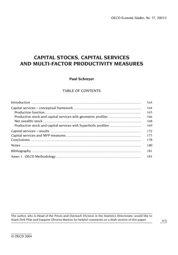
Capital Stocks, Capital Services and Multi-factor Productivity Measurescapital services, the wealth (net) stock measures the market value of capitalassets. “Wealth stock” is sometimes considered a more precise terminology, however, because there are other forms of “net” stock, in particular the productivestock which is a stock “net” of efficiency declines in productive assets. In thepresent setting, the net stock at current prices is obtained by valuing each asset’sproductive stock by the market price of the corresponding new asset. The totalvalue of the net stock is obtained by adding the individual values of eachasset: qtWt i qti Sti 1 i qti K ti .The rate of change of the net stock at constant prices depends again on theindex number formula chosen for aggregation across assets. One obvious possibilityis to employ again a Törnqvist-type formula to obtain:ln(Wt 1 Wt ) i 0.5( wti 1 wti ) ln(Wt i 1 Wt i )wherewti qti, 0 K ti qiit ,0K ti[5]Because the net stock is a concept that is well anchored in the system ofnational accounts, most OECD countries publish data for a net stock of fixedassets. However, these series are not normally aggregated through Törnqvist indices: the majority of countries use a Laspeyres-type volume index7 which introduces an additional difference between measures of capital stocks available fromthe national accounts and measures of capital services for productivity analysis.To conclude, there are two key features that distinguish the rate of change ofthe capital services measure from that of the net capital stock: the weightingscheme and in many cases the index number formula used. In periods of rapidchange of relative prices and volumes both elements contribute to potentially significant differences between the time profiles of the two measures. Usage of thenet stock in productivity computations instead of the capital services measure canthen give rise to a biased statistic of multi-factor productivity. To illustrate,Figure 1 below compares the two measures for the United States and for Franceand Box 2 provides a numerical example.Productive stock and capital services with hyperbolic profilesThe use of geometric patterns to describe the efficiency and price profiles ofassets is computationally convenient. Also, there is empirical evidence for priceprofiles that resemble geometric patterns. Everyday experience suggests that theprices of assets decline by relatively large absolute amounts in the first years aftertheir purchase – a 20 per cent drop in the value of a new car during its first year of OECD 2004169
OECD Economic Studies No. 37, 2003/2Figure 1. Capital services and net capital stock1Capital servicesNet capital stock180160United 001. Based on geometric age-efficiency and age-price profile and “harmonised” ICT deflators. Aggregation throughTörnqvist indices.Source: Derived from OECD Capital Services Database (October 2003).usage is a well-know empirical phenomenon. However, is the same pattern plausible when it comes to describing the relative efficiency of a vintage product? Forexample, does a car loose one fifth of its capacity to generate transport servicesduring its first year of usage? Based on a single capital item, the answer to thisquestion will often be “no” and this suggests adopting an approach that allows fordifferences in the efficiency and in the price profiles of assets while keeping thetwo profilesconsistent.170The OECD capital services measure is based on a hyperbolic pattern for itsefficiency profile and derives a consistent price profile. A hyperbolic patternassumes a slow loss in productive efficiency over the first years of an asset’s service life and a more rapid decline towards the end of the service life. This is shownin Figure 2. It reproduces the age-efficiency profile for transport equipment – anasset whose average service life is taken to be 15 years. Neither the hyperbolicnor the geometric pattern breaks off at the 15 years. In the case of the hyperboliccurve, an assumption has been made that retirement of a cohort is distributedaround the median service life of 15 years. In the case of the geometric pattern, noexplicit retirement function is formulated. It is assumed that the geometric declinecaptures both the effects of wear and tear and retirement. OECD 2004
Capital Stocks, Capital Services and Multi-factor Productivity MeasuresBox 2.Wealth stock and capital services in the presence of technicalchange – a numerical exampleThe choice of aggregation weights becomes crucial when prices and quantities of different types of capital goods evolve at very different rates. This is, forexample, the case when there is relatively rapid quality change of one type ofasset compared with others. Aggregation of assets by way of purchase prices willgenerate a serious bias in the capital input measures because purchase prices willinadequately approximate the marginal productivity of assets which constitutethe appropriate weights for aggregation of capital services. User costs aredesigned to reflect the marginal productivity of assets: capital goods areemployed until their marginal revenue (itself dependent on marginal productivity) equals marginal cost (the user cost or rental price) of an asset. The differencebetween purchase prices (q) and user costs (uc) is the gross rate of return (GRR)that an asset must yield per year: uc q*GRR. The gross rate of return itself iscomposed of the net rate of return, the rate of depreciation and rate of revaluation or asset price change. Rapid negative price changes or large rates of depreciation therefore imply large gross rates of return and user costs. Thus, anaggregation based on user cost weights will give more weight to assets with relatively large GRRs as opposed to an aggregation based on purchase prices, q.Consider the following example with two assets, A and B. In period t 0, thepurchase price of both assets equals unit but declines by 30 per cent in the caseof A and rises by 10 per cent in the case of B. Given the quantities of investmentand the (geometric) rates of depreciation, a capital stock in period t 1 can easilybe calculated. In the present case, wealth and productive stock coincide at thelevel of individual assets. Assume a net rate of return of 5 per cent. The total usercost is then computed as 0.55 for Asset A and 0.15 for Asset B. This gives rise to ashare of Asset A in total user costs in period t 0 of 79 per cent and a share ofAsset B of 21 per cent – quite different from the 50 per cent share for each assetwhen weights are based on purchase prices. Finally, construct a simple Laspeyresquantity index of capital services and the wealth stock and it is easy to see thatthe former rises much faster than the latter.Asset APurchase pricet 0t 1Quantity of Investmentt 0t 1Productive stock/Wealth stock t 0t 1User costsWeights t 0Laspeyres quantity indexNet rate of returnDepreciationRevaluationTotalUser cost basedPurchase price basedUser cost basedPurchase price basedAsset .500.050.200.100.150.210.502.151.95171 OECD 2004
OECD Economic Studies No. 37, 2003/2Figure 2. Hyperbolic and geometric age-efficiency patternAverage service life 15 921Capital services measures are sensitive to the choice of the age-efficiencyprofile. For example, capital services measures based on geometric age-efficiencyprofiles rise by 1.5 per cent per year on average in Australia over the period 1985-01.The same variable based on hyperbolic profiles grows at 2.2 per cent per year.Similarly, the geometrically-based series for the United States exhibits a 3.4 percent growth rate over the same period whereas the hyperbolic pattern produces agrowth rate close to 4 per cent. In France, the figures are 2.5 per cent per year(geometric) and 3.1 per cent per year (hyperbolic).CAPITAL SERVICES – RESULTS172The following section presents a set of capital service measures for the G-7countries and Australia. The results presented are based on a more generalmodel than the one set out in the second section of this paper. In particular, efficiency profiles were not assumed to be geometric. Results based on geometricprofiles are also available from the database but as a special case. To start out,Table 1 shows the volume changes of capital services, by type of asset or by typeof product. At the level of individual assets, the rate of change of capital services isjust equal to the evolution of the productive stock. The aggregate index of capitalservices (Table 2) corresponds to a weighted average of the each asset’s index of OECD 2004
Capital Stocks, Capital Services and Multi-factor Productivity MeasuresTable 1. Volume growth of capital services by type of asset1Compound annual percentage changes, total economy, based on “harmonised” deflators for ICT assetsProducts of agriculture metalproducts and ther .21. Using a hyperbolic age-efficiency profile.Source: OECD capital services data base (October 2003).capital services where nominal shares in total user costs constitute the relevantweights.Rates of change of deflators can be found in Table 3. To account for some ofthe methodological differences between countries’ deflators for information andcommunication technology products, the results presented here are based on“harmonised” deflators (see Box 3).A first way of assessing the set of capital services measures produced here isto compare them with similar data published at the national level. Today, this possibility for comparison exists only for a few countries. These are Australia (ABSpublishes capital services data as part of its annual national accounts), the United OECD 2004173
OECD Economic Studies No. 37, 2003/2Table 2. Volume index of capital services (all assets)11980 100, total economy, based on “harmonised’ deflators for ICT 3165.6173.2182.8194.1206.4218.5227.51. Using a hyperbolic age-efficiency profile.Source: OECD capital services data base (October 2003).States (capital services series are published by the Bureau of Labor Statistics aspart of its multifactor productivity measurement programme) and the UnitedKingdom where work is underway at ONS and where a first set of capital servicesdata has been published at the Bank of England (Oulton 2001). Statistics Canadahas also compiled a set of capital services measures (Harchaoui and Tarkhani2002) and work is underway in Spain (Mas et al. 2002).174A first comparison of our results for Australia and those published by theAustralian Bureau of Statistics8 reveals two points. First, the time profile of theOECD series follows that of the ABS series fairly closely. At the same time, andthis is the second observation, there appears to be a systematic downward bias(5.1 versus 3.7 per cent per year between 1980 and 1999) of the OECD measureswith regard to the official statistics. This is, however, due to the fact that the ABSseries relates to the business sector whereas our results concern the entire economy. When only private sector data are used in the OECD model, a capital servicemeasure with similar rates of change to those of the official ABS time series isfound. Other small sources of differences in methodology persist (e.g. ABS chooses OECD 2004
Capital Stocks, Capital Services and Multi-factor Productivity MeasuresTable 3. Price indices of capital goods by type of asset1Compound annual percentage changes, total economy, based on “harmonised’ ICT deflatorsProducts of agriculture, metalproducts and machineryHardwareCommunicationEquipmentOther –0.2–2.53.73.52.53.03
Capital services are an integral part of a durable goods model of production,itself characterised by a production function, say G that is separable in the ser-vices of different vintages of different types of capital goods: Q GKK K N t ( t[,K t,.,],L,t) [1] tt NIn(1), KK K [,,.,K]is an aggregator of capital services from N different