Transcription
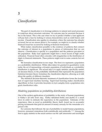
3ClassificationThe goal of classification is to leverage patterns in natural and social processesto conjecture about uncertain outcomes. An outcome may be uncertain because itlies in the future. This is the case when we try to predict whether a loan applicantwill pay back a loan by looking at various characteristics such as credit history andincome. Classification also applies to situations where the outcome has alreadyoccurred, but we are unsure about it. For example, we might try to classify whetherfinancial fraud has occurred by looking at financial transaction.What makes classification possible is the existence of patterns that connectthe outcome of interest in a population to pieces of information that we canobserve. Classification is specific to a population and the patterns prevalent inthe population. Risky loan applicants might have a track record of high creditutilization. Financial fraud often coincides with irregularities in the distribution ofdigits in financial statements. These patterns might exist in some contexts but notothers.We formalize classification in two steps. The first is to represent a populationas a probability distribution. While often taken for granted in quantitative worktoday, the act of representing a dynamic population of individuals as a probabilitydistribution is significant. The second step is to apply statistics, specifically statistical decision theory, to the probability distribution that represents the population.Statistical decision theory formalizes the classification objective, allowing us to talkabout the quality of different classifiers.The statistical decision-theoretic treatment of classification forms the foundation of supervised machine learning. Supervised learning makes classificationalgorithmic in how it provides heuristics to turn samples from a population intogood classification rules.Modeling populations as probability distributionsOne of the earliest applications of probability to the study of human populationsis Halley’s life table from 1693. Halley tabulated births and deaths in a smalltown in order to estimate life expectancy in the population. Estimates of lifeexpectancy, then as novel as probability theory itself, found use in accuratelypricing investments that paid an amount of money annualy for the remainder of aperson’s life.For centuries that followed, the use of probability to model human populations,however, remained contentious both scientifically and politically.1, 2, 3 Among thefirst to apply statistics to the social sciences was the 19th astronomer and sociologist1
Figure 1: Halley’s life table (1693)Adolphe Quetelet. In a scientific program he called “social physics”, Queteletsought to demonstrate the existence of statistical laws in human populations. Heintroduced the concept of the “average man” characterized by the mean values ofmeasured variables that followed a normal distribution. As much a descriptive as anormative proposal, Quetelet regarded averages as an ideal to be pursued. Amongothers, his work influenced Francis Galton in the development of eugenics.The success of statistics throughout the 20th century cemented in the use ofprobability to model human populations. Few raise an eyebrow today if we talkabout a survey as sampling responses from a distribution. It seems obvious nowthat we’d like to estimate parameters such as mean and standard deviation fromthis distribution. Statistics is so deeply embedded in the social sciences that werarely revisit the premise that we can represent a human population as a probabilitydistribution.The differences between a human population and a distribution are stark. Human populations change over time, sometimes rapidly, due to different mechanismsand interactions among individuals. A distribution, in contrast, can be thought ofas a static array where rows correspond to individuals and columns correspond tomeasured covariates of an individual. The mathematical abstraction for such anarray is a set of nonnegative numbers, called probabilities, that sum up 1 and giveus for each row the relative weight of this setting of covariates in the population.To sample from a such a distribution corresponds to picking one of the rows in thetable at random in proportion to its weight. We can repeat this process withoutchange or deteriation.Much of statistics deals with samples and the question how we can relatequantities computed on a sample, such as the sample avearge, to correspondingparameters of a distribution, such as the population mean. The focus in ourchapter is different. We’ll use statistics to talk about properties of populations asdistributions and by extension classification rules applied to a population. While2
sampling introduces many additional issues, the questions we raise in this chaptercome out most clearly at the population level.Formalizing classificationThe goal of classification is to determine a plausible value for an unknown targetY given observed covariates X. Formally, the covariates X and target Y are jointlydistributed random variables. This means that there is one probability distributionover pairs of values ( x, y) that the random variables ( X, Y ) might take on. Thisprobability distribution models a population of instances of the classificationproblem. In most of our examples, we think of each instance as the covariates andtarget of one individual.At the time of classification, the value of the target variable is not known tob f ( X ) based on whatus, but we observe the covariates X and make a guess Yb is calledwe observed. The funtion f that maps our covariates into our guess Ya classifier. The output of the classifier is sometimes called a prediction or label.bThroughout this chapter we are primarily interested with the random variable Yand how it relates to other random variables. The function that defines this randomvariables is secondary. For this reason, we stretch the terminology slightly andb itself as the classifier.refer to YWhat makes a classifier good for an application and how do we choose one outof many possible classifiers? This question often does not have a fully satisfyinganswer, but statistical decision theory provides criteria can help highlight differentqualities of a classifier that can inform our choice.b is its classificationPerhaps the most well known property of a classifier Ybaccuracy, or accuracy for short, defined as P{Y Y }, the probability of correctlyb}. Accuracypredicting the target variable. We define classification error as P{Y 6 Yis easy to define, but misses some important aspects when evaluating a classifier.A classifier that always predicts no traffic fatality in the next year might have highaccuracy on any given individual, simply because fatal accidents are unlikely.However, it’s a constant function that has no value in assessing the risk of a trafficfatality.Other decision-theoretic criteria highlight different aspects of a classifier. Wecan define the most common ones by considering the conditional probabilityP{event condition} for various different settings.Table 1: Common classification criteriaEventbYbYbYbY 1 0 1 0ConditionYYYY 1 1 0 0Resulting notion (P{event condition})True positive rate, recallFalse negative rateFalse positive rateTrue negative rate3
The true positive rate corresponds to the frequency with which the classifiercorrectly assigns a positive label when the outcome is positive. We call this atrue positive. The other terms false positive, false negative, and true negative deriveanalogously from the respective definitions. It is not important to memorize allthese terms. They do, however, come up regularly in the classification settings.Another family of classification criteria arises from swapping event and condition. We’ll only highlight two of the four possible notions.Table 2: Additional classification criteriaEventConditionY 1Y 0b 1Yb 0YResulting notion (P{event condition})Positive predictive value, precisionNegative predictive valueOptimal classificationSuppose we assign a cost (or reward) to each of the four possible classificationoutcomes, true positive, false positive, true negative, false negative. The problem ofoptimal classification is to find a classifier that minimizes cost in expectation overa population. We can write the cost as a real number (yb, y) that we experiencewhen we classify a target value y with a label yb. An optimal classifier is any classifierthat minimizes the objective:b Y )]E[ (Y,This objective is called classification risk and risk minimization refers to the optimization problem of finding a classifier that minimizes risk.As an example, choose (0, 1) (1, 0) 1 and (1, 1) (0, 0) 0. For thisloss function, the optimal classifier is the one that minimizes classification error.The resulting optimal classifier has an intuitive solution.Fact 1. The optimal predictor minimizing classification error satisfies(b f ( X ) , where f ( x ) 1 if P{Y 1 X x } 1/2Y0 otherwise.The optimal classifier checks if the propensity of positive outcomes given theobserved covariates X is greater than 1/2. If so, it makes the guess that the outcomeis 1. Otherwise, it guesses that the outcome is 0. Although the optimal predictoris specific to classicication error, it extends to the general case by varying thethreshold. This makes intuitive sense. If our cost for false positives was muchhigher than our cost for false negatives, we’d better err on the side of not declaringa positive.4
Risk scoresThe optimal classifier we just saw has an important property. We were able to writeit as a threshold applied to the functionr ( x ) P {Y 1 X x } E [Y X x ] .This function is an example of a risk score. Statistical decision theory tells us thatoptimal classifiers can generally be written as a threshold applied to this risk score.The risk score we see here is a particularly important and natural one. We canthink of it as taking the available evidence X x and calculating the expectedoutcome given the observed information. This is called the posterior probability of Ygiven X. In an intuitive sense, the conditional expectation is a statistical lookup tablethat gives us for each setting of features the frequency of positive outcomes giventhese features.The risk score is in itself optimal in that it minimizes the squared lossE(Y r ( X ))2among all possible real-valued risk scores r ( X ). Minimization problems where wetry to approximate the target variable Y with a real-valued risk score are calledregression problems. In this context, risk scores are often called regressors.Although our loss function was specific, there is a general lesson. Classificationis often attacked by first solving a regression problem to summarize the data ina single real-valued risk score. We then turn the risk score into a classifier bythresholding.Risk scores need not be optimal or learned from data. For an illustrativeexample consider the well-known body mass index, due to Quetelet by the way,which summarizes weight and height of a person into a single real number. In ourformal notation, the features are X ( H, W ) where H denotes height in metersand W denotes weight in kilograms. The body mass index corresponds to the scorefunction R W/H 2 .We could interpret the body mass index as measuring risk of, say, diabetes.Thresholding it at the value 30, we might decide that individuals with a bodymass index above this value are at risk of developing diabetes while others arenot. It does not take a medical degree to worry that the resulting classifier maynot be very accurate. The body mass index has a number of known issues leadingto errors when used for classification. We won’t go into detail, but it’s worthnoting that these classification errors can systematically align with certain groupsin the population. For instance, the body mass index tends to be inflated as a riskmeasure for taller people due to scaling issues.A more refined approach to finding a risk score for diabetes would be to solvea regression problem involing the available covariates and the outcome variable.Solved optimally, the resulting risk score would tell us for every setting of weight(say, rounded to the nearest kg unit) and every physical height (rounded to thenearest cm unit), the incidence rate of diabetes among individuals with thesevalues of weight and height. The target variable in this case is a binary indicator of5
Figure 2: Plot of the body mass index.diabetes. So, r ((176, 68)) would be the incidence rate of diabetes among individualswho are 1.76m tall and weigh 68kg. The conditional expectation is likely moreuseful as a risk measure of diabetes than the body mass index we saw earlier. Afterall, the conditional expectation directly reflects the incidence rate of diabetes giventhe observed characteristics, while the body mass index didn’t solve this specificclassification problem.Varying thresholds and ROC curvesIn the optimal predictor for classification error we chose a threshold of 1/2. Thisexact number was a consequence of the equal cost for false positives and falsenegatives. If a false positive was significantly more costly, we might wish to choosea higher threshold for declaring a positive. Each choice of a threshold results in aspecific trade-off between true positive rate and false positive rate. By varying thetreshold from 0 to 1, we can trace out a curve in a two-dimensional space wherethe axes correspond to true positive rate and false positive rate. This curve is calledan ROC curve. ROC stands for receiver operator characteristic, a name pointing atthe roots of the concept in signal processing.We can achieve any trade-off below the ROC curve via randomization. Tounderstand this point, think about how we can realize trade-offs on the the dashedline in the plot. Take one classifier that accepts everyone. This corresponds to trueand false positive rate 1, hence achieving the upper right corner of the plot. Takeanother classifier that accepts no one, resulting in true and false positive rate 0,the lower left corner of the plot. Now, construct a third classifier that given aninstance randomly picks and applies the first classifier with probability 1 p, andthe second with probability p. This classifier achieves true and false positive rate pthus giving us one point on the dashed line in the plot. In the same manner, we6
Figure 3: Example of an ROC curvecould have picked any other pair of classifiers and randomized between them. Thisway we can realize the entire area under the ROC curve. In particular, this meansthe area under the ROC curve must be convex, meaning that every point in it lieson a line segment between two classifiers on the boundary.Strictly speaking, in statistical decision theory, the ROC curve is a property of adistribution ( X, Y ). It gives us for each setting of false positive rate, the optimaltrue positive rate that can be achieved for the given false positive rate on thedistribution ( X, Y ). This leads to several nice theoretical properties of the ROCcurve. In the machine learning context, ROC curves are computed more liberallyfor any given risk score, even if it isn’t optimal. The ROC curve is often used toeyeball how predictive our score is of the target variable. A common measure ofpredictiveness is the area under the curve (AUC), which equals the probability thata random positive instance gets a score higher than a random negative instance.An area of 1/2 corresponds to random guessing, and an area of 1 corresponds toperfect classification.Supervised learningSupervised learning is what makes classification algorithmic. It instructs us how toconstruct good classifiers from samples drawn from a population. The details ofsupervised learning won’t matter for this chapter, but it is still worthwhile to havea working understanding of the basic idea.Suppose we have labeled data, also called training examples, of the form( x1 , y1 ), ., ( xn , yn ), where each example is a pair ( xi , yi ) of an instance xi and alabel yi . We typically assume that these examples were drawn independently andrepeatedly from the same distribution ( X, Y ). A supervised learning algorithm7
takes in training examples and returns a classifier, typically a threshold of ascore: f ( x ) 1{r ( x ) t}. A simple example of a learning algorithm is the familiarleast squares method that attempts to minimize the objective functionn (r ( xi ) yi )2.i 1We saw earlier that at the population level, the optimal score is the conditionalexpectation r ( x ) E [Y X x ] . The problem is that we don’t necessarily haveenough data to estimate each of the conditional probabilities required to constructthis score. After all, the number of possible values that x can assume is exponentialin the number of covariates.The whole trick in supervised learning is to approximate this optimal solutionwith algorithmically feasible solutions. In doing so, supervised learning mustnegotiate a balance along three axes: Representation: Choose a family of functions that the score r comes from.A common choice are linear functions r ( x ) hw, x i for some vector ofcoefficients w. More complex representations involve non-linear functions,such as artificial neural networks. This function family is often called the modelclass and the coefficients w are called model parameters. Optimization: Solve the resulting optimization problem by finding modelparameters that minimize the loss function on the training examples. Generalization: Argue why small loss on the training examples implies smallloss on the population that we drew the training examples from.The three goals of supervised learning are entangled. A powerful representationmight make it easier to express complicated patterns, but it might also burdenoptimization and generalization. Likewise, there are tricks to make optimizationfeasible at the expense of representation or generalization.For the remainder of this chapter, we can think of supervised learning as a blackbox that provides us with classifiers when given training data. What matters arewhich properties these classifiers have at the population level. At the populationb f ( X ). Welevel, we interpret a classifier as a random variable by considering Ybignore how Y was learned from a finite sample, what the functional form of theclassifier is, and how we estimate various statistical quantities from finite samples.While finite sample considerations are fundamental to machine learning, they arenot central to the conceptual and technical questions around fairness that we willdiscuss in this chapter.Protected categoriesChapter 2 introduced some of the reasons why individuals might want to object tothe use of statistical classification rules in consequential decisions. We now turnto one specific concern, namely, discrimination on the basis of membership in specific8
groups of the population. Discrimination is not a general concept. It is concernedwith socially salient categories that have served as the basis for unjustified andsystematically adverse treatment in the past. United States law recognizes certainprotected categories including race, sex (which extends to sexual orientation), religion,disability status, and place of birth.In many classification tasks, the features X implicitly or explicitly encodeand individual’s status in a protected category. We will set aside the letter Ato designate a discrete random variable that captures one or multiple sensitivecharacteristics. Different settings of the random variable A correspond to differentmutually disjoint groups of the population. The random variable A is often calleda sensitive attribute in the technical literature.Note that formally we can always represent any number of discrete protectedcategories as a single discrete attribute whose support corresponds to each of thepossible settings of the original attributes. Consequently, our formal treatment inthis chapter does apply to the case of multiple protected categories.The fact that we allocate a special random variable for group membership doesnot mean that we can cleanly partition the set of features into two independentcategories such as “neutral” and “sensitive”. In fact, we will see shortly that sufficiently many seemingly neutral features can often give high accuracy predictionsof group membership. This should not be surprising. After all, if we think of A asthe target variable in a classification problem, there is reason to believe that theremaining features would give a non-trivial classifier for A.The choice of sensitive attributes will generally have profound consequences asit decides which groups of the population we highlight, and what conclusions wedraw from our investigation. The taxonomy induced by discretization can on itsown be a source of harm if it is too coarse, too granular, misleading, or inaccurate.The act of classifying status in protected categories, and collecting associated data,can on its own can be problematic. We will revisit this important discussion in thenext chapter.No fairness through unawarenessSome have hoped that removing or ignoring sensitive attributes would somehowensure the impartiality of the resulting classifier. Unfortunately, this practice canbe ineffective and even harmful.In a typical dataset, we have many features that are slightly correlated with thesensitive attribute. Visiting the website pinterest.com, for example, has a smallstatistical correlation with being female.1 The correlation on its own is too small topredict someone’s gender with high accuracy. However, if numerous such featuresare available, as is the case in a typical browsing history, the task of predictinggender becomes feasible at high accuracy levels.Several features that are slightly predictive of the sensitive attribute can be usedto build high accuracy classifiers for that attribute. In large feature spaces sensitive1 Asof August 2017, 58.9% of Pinterest’s users in the United States were female. See here (Retrieved3-27-2018)9
Figure 4: On the left, we see the distribution of a single feature that differs onlyvery slightly between the two groups. In both groups the feature follows a normaldistribution. Only the means are slightly different in each group. Multiple featureslike this can be used to build a high accuracy group membership classifier. On theright, we see how the accuracy grows as more and more features become available.attributes are generally redundant given the other features. If a classifier trainedon the original data uses the sensitive attribute and we remove the attribute, theclassifier will then find a redundant encoding in terms of the other features. Thisresults in an essentially equivalent classifier, in the sense of implementing the samefunction.To further illustrate the issue, consider a fictitious start-up that sets out topredict your income from your genome. At first, this task might seem impossible.How could someone’s DNA reveal their income? However, we know that DNAencodes information about ancestry, which in turn correlates with income in somecountries such as the United States. Hence, DNA can likely be used to predictincome better than random guessing. The resulting classifier uses ancestry inan entirely implicit manner. Removing redundant encodings of ancestry fromthe genome is a difficult task that cannot be accomplished by removing a fewindividual genetic markers. What we learn from this is that machine learning canwind up building classifiers for sensitive attributes without explicitly being askedto, simply because it is an available route to improving accuracy.Redundant encodings typically abound in large feature spaces. What aboutsmall hand-curated feature spaces? In some studies, features are chosen carefullyso as to be roughly statistically independent of each other. In such cases, thesensitive attribute may not have good redundant encodings. That does not meanthat removing it is a good idea. Medication, for example, sometimes depends onrace in legitimate ways if these correlate with underlying causal factors.4 Forcingmedications to be uncorrelated with race in such cases can harm the individual.10
Statistical non-discrimination criteriaStatistical non-discrimination criteria aim to define the absence of discriminationin terms of statistical expressions involving random variables describing a classification or decision making scenario.Formally, statistical non-discrimination criteria are properties of the joint distribub or score R,tion of the sensitive attribute A, the target variable Y, the classifier Yand in some cases also features X. This means that we can unambiguously decidewhether or not a criterion is satisfied by looking at the joint distribution of theserandom variables.Broadly speaking, different statistical fairness criteria all equalize some groupdependent statistical quantity across groups defined by the different settings of A.For example, we could ask to equalize acceptance rates across all groups. Thiscorresponds to imposing the constraint for all groups a and b:b 1 A a } P {Yb 1 A b} .P {Yb {0, 1} is a binary classifier and we have two groups aIn the case where Yand b, we can determine if acceptance rates are equal in both groups by knowingb 1, A a}, P{Yb 1, A b}, and P{ A a} thatthe three probabilities P{Ybfully specify the joint distribution of Y and A. We can also estimate the relevantprobabilities given random samples from the joint distribution using standardstatistical arguments that are not the focus of this chapter.Researchers have proposed dozens of different criteria, each trying to capturedifferent intuitions about what is fair. Simplifying the landscape of fairness criteria,we can say that there are essentially three fundamentally different ones. Each ofthese equalizes one of the following three statistics across all groups:b 1} of a classifier Yb Acceptance rate P{Ybbb Error rates P{Y 0 Y 1} and P{Y 1 Y 0} of a classifier Y Outcome frequency given score value P{Y 1 R r } of a score RThe three criteria can be generalized and simplified using three different (conditional) independence statements. We use the notation U V W to denotethat random variables U and V are conditionally independent given W.2 Thismeans that conditional on any setting W w, the random variables U and V areindependent.Table 3: Non-discrimination criteria2 Wasserman’sIndependenceSeparationSufficiencyR AR A YY A Rtext5 gives an excellent introduction to conditional independence and its properties.11
Below we will introduce and discuss each of these conditions in detail. Variantsof these criteria arise from different ways of relaxing them. Earlier on we used theb for a classifier. To avoid notational clutter, we think of a binary classifierletter Ynow as a special case of a score function R {0, 1} that has just two values.This chapter focuses on the mathematical properties of and relationships between these different criteria. Once we have acquired familiarity with the technicalmatter, we’ll have a broader debate around the moral and normative content ofthese definitions in Chapter 4.IndependenceOur first formal criterion requires the sensitive characteristic to be statisticallyindependent of the score.Definition 1. Random variables ( A, R) satisfy independence if A R.Independence has been explored through many equivalent terms or variants,referred to as demographic parity, statistical parity, group fairness, disparate impact andothers. In the case of binary classification, independence simplifies to the conditionP{ R 1 A a } P{ R 1 A b } ,for all groups a, b. Thinking of the event R 1 as “acceptance”, the conditionrequires the acceptance rate to be the same in all groups. A relaxation of theconstraint introduces a positive amount of slack e 0 and requires thatP{ R 1 A a } P{ R 1 A b } e .Note that we can swap a and b to get an inequality in the other direction. Analternative relaxation is to consider a ratio condition, such as,P{ R 1 A a } 1 e.P{ R 1 A b }Some have argued that, for e 0.2, this condition relates to the 80 percent rule thatappears in discussions around disparate impact law.6Yet another way to state the independence condition in full generality is torequire that A and R must have zero mutual information I ( A; R) 0. Mutualinformation quantifies the amount of information that one random variable revealsabout the other. We can define it in terms of the more standard entropy functionas I ( A; R) H ( A) H ( R) H ( A, R). The characterization in terms of mutualinformation leads to useful relaxations of the constraint. For example, we couldrequire I ( A; R) e.12
Limitations of independenceIndependence is pursued as a criterion in many papers, for multiple reasons. Someargue that the condition reflects an assumption of equality: All groups have anequal claim to acceptance and resources should therefore be allocated proportionally. What we encounter here is a question about the normative significance ofindependence, which we extend on in Chapter 4. But there is a more mundane reason for the prevalence of this criterion, too. Independence has convenient technicalproperties, which makes the criterion appealing to machine learning researchers. Itis often the easiest one to work with mathematically and algorithmically.However, decisions based on a classifier that satisfies independence can haveundesirable properties (and similar arguments apply to other statistical critiera).Here is one way in which this can happen, which is easiest to illustrate if weimagine a callous or ill-intentioned decision maker. Imagine a company that ingroup a hires diligently selected applicants at some rate p 0. In group b, thecompany hires carelessly selected applicants at the same rate p. Even though theacceptance rates in both
tion of supervised machine learning. Supervised learning makes classification algorithmic in how it provides heuristics to turn samples from a population into good classification rules. Modeling populations as probability distributions One of the earliest applications of probability to the study of human populations is Halley's life table .