WIXLIB

individualproblemTable 1: Summary of notations for individuals vs. problemsspace element distributiondata setsample size empirical dist.b U (X)PXx XPX {xi }nni 1Ff FF {fj }mj 1Qmb U (F )Q2. Fairness: with probability 1 β over the draw of new individuals x, x0 P, the error rate(or false positive or negatives rates) of the output mapping (computed in expectation overproblems f Q) on x will be within O(α) of that of x0 .The mapping from new classification problems to hypotheses that we find is derived from the dualvariables of the linear program representing our empirical risk minimization task, and we cruciallyrely on the structure of this mapping to prove our generalization guarantees for new problems f Q.1.2Additional related workThe literature on fairness in machine learning has become much too large to comprehensivelysummarize, but see Mitchell et al. (2018) for a recent survey. Here we focus on the most conceptuallyrelated work, which has aimed to bridge the gap between the immediate applicability of statisticaldefinitions of fairness with the strong individual level semantics of individual notions of fairness.One strand of this literature focuses on the “metric fairness” definition first proposed by Dwork et al.(2012), and aims to ease the assumption that the learning algorithm has access to a task specificfairness metric. Kim et al. (2018a) imagine access to an oracle which can provide unbiased estimatesto the metric distance between any pair of individuals, and show how to use this to satisfy a statisticalnotion of fairness representing “average metric fairness” over pre-defined groups. Gillen et al. (2018)study a contextual bandit learning setting in which a human judge points out metric fairness violationswhenever they occur, and show that with this kind of feedback (under assumptions about consistencywith a family of metrics), it is possible to quickly converge to the optimal fair policy. Yona andRothblum (2018) consider a PAC-based relaxation of metric fair learning, and show that empiricalmetric-fairness generalizes to out-of-sample metric fairness. Another strand of this literature hasfocused on mitigating the problems that arise when statistical notions of fairness are imposed overcoarsely defined groups, by instead asking for statistical notions of fairness over exponentially manyor infinitely many groups with a well defined structure. This line includes Hébert-Johnson et al.(2018) (focusing on calibration), Kearns et al. (2018) (focusing on false positive and negative rates),and Kim et al. (2018b) (focusing on error rates).2Model and preliminariesWe model each individual in our framework by a vector of features x X , and we let each learningproblem 1 be represented by a binary function f F mapping X to {0, 1}. We assume probabilitymeasures P and Q over X and F, respectively. In the training phase there is a fixed (across problems)set X {xi }ni 1 of n individuals sampled independently from P for which we have available labels2corresponding to m tasks represented by F {fj }mj 1 drawn independently from Q . Therefore, amtraining data set of n individuals X and m learning tasks F takes the form: S {xi , (fj (xi ))j 1 }ni 1 .We summarize the notations we use for individuals and problems in Table 1.In general F will be unknown. We will aim to solve the (agnostic) learning problem over a hypothesisclass H, which need bear no relationship to F. We will allow for randomized classifiers, which wemodel as learning over (H), the probability simplex over H. We assume throughout that H containsthe constant classifiers h0 and h1 where h0 (x) 0 and h1 (x) 1 for all x. Unlike usual learningsettings where the primary goal is to learn a single hypothesis p (H), our objective is to learn amapping ψ (H)F that maps learning tasks f F represented as new labellings of the trainingdata to hypotheses p (H). We will therefore have to formally define the error rates incurredby a mapping ψ and use them to formalize a learning task subject to our proposed fairness notion.For a mapping ψ, we write ψf to denote the classifier corresponding to f under the mapping, i.e.,12We will use the terms: problem, task, and labeling interchangeably.Throughout we will use subscript i to denote individuals and j to denote learning problems.3

ψf ψ (f ) (H). Notice in the training phase, there are only m learning problems to be solved,and therefore, the corresponding empirical problem reduces to learning m randomized classifiers.In general, learning m specific classifiers for the training problems will not yield any generalizablerule mapping new problems to classifiers — but the specific algorithm we propose for empirical riskminimization will induce such a mapping, via a dual representation of the empirical risk minimizer.FDefinition 2.1 (Individual and OverallError Rates). For a mapping ψ (H) and distributionsP and Q: E (x, ψ; Q) Ef Q Ph ψf [h(x) 6 f (x)] is the individual error rate of x incurred byψ and err (ψ; P, Q) E [E (x, ψ; Q)] is the overall error rate of ψ.x PIn the body of this paper, we will focus on a fairness constraint that asks that the individual errorrate should be approximately equalized across all individuals. In the supplement, we extend ourtechniques to equalizing false positive and negative rates across individuals.Definition 2.2 (Average Individual Fairness (AIF)). We say a mapping ψ (H)F satisfies “(α, β)AIF” (reads (α, β)-approximate Average Individual Fairness) with respect to the distributions (P, Q)if there exists γ 0 such that: Px P ( E (x, ψ; Q) γ α) β.We briefly fix some notation: 1 [A] represents the indicator function of event A. For n N,[n] {1, 2, . . . , n}. U (S) represents the uniform distribution over S. For a mapping ψ : A Band A0 A, ψ A0 represents ψ restricted to the domain A0 . dH denotes the VC dimension of theclass H. CSC(H) denotes a cost sensitive classification oracle for H:Definition 2.3 (Cost Sensitive Classification (CSC) in H). Let D {xi , c1i , c0i }ni 1 denote adata set of n individuals xi where c1i and c0i are the costs of classifying xi as positive (1) andnegative (0) respectively. Given D, thePcost sensitiveclassification problem defined over H isn the optimization problem: arg minh H i 1 c1i h(xi ) c0i (1 h(xi )) . An oracle CSC(H)takes D {xi , c1i , c0i }ni 1 as input and outputs the solution to the optimization problem. We useCSC(H; D) to denote the classifier returned by CSC(H) on data set D. We say that an algorithmis oracle efficient if it runs in polynomial time given the ability to make unit-time calls to CSC(H).3Learning subject to AIFIn this section we first cast the learning problem subject to the AIF fairness constraints as theconstrained optimization problem (1) and then develop an oracle efficient algorithm for solving itscorresponding empirical risk minimization (ERM) problem (in the spirit of Agarwal et al. (2018)).In the coming sections we give a full analysis of the developed algorithm including its in-sampleaccuracy/fairness guarantees and define the mapping it induces from new problems to hypotheses,and finally establish out-of-sample bounds for this trained mapping.Fair Learning Problem subject to (α, 0)-AIFminψ (H)F , γ [0,1]s.t. x X :err (ψ; P, Q)(1) E (x, ψ; Q) γ αDefinition 3.1 (OPT). Consider the optimization problem (1). Given distributions P and Q, andfairness approximation parameter α, we denote the optimal solutions of (1) by ψ ? (α; P, Q) andγ ? (α; P, Q), and the value of the objective function at these optimal points by OPT (α; P, Q).We will use OPT as the benchmark with respect to which we evaluate the accuracy of our trainedmapping. It is worth noticing that the optimization problem (1) has a nonempty set of feasiblesolutions for every α and all distributions P and Q because the following point is always feasible:γ 0.5 and ψf 0.5h0 0.5h1 (i.e. random classification) for all f F where h0 and h1 areall-zero and all-one constant classifiers.3.1The empirical fair learning problemWe start to develop our algorithm by defining the empirical version of (1) for a given training dataset of n individuals X {xi }ni 1 and m learning problems F {fj }mj 1 . We will formulate the4

empirical problem as finding a restricted mapping ψ F by which we mean the domain of the mappingis restricted to the training set F F. We will later see how the dynamics of our proposed algorithmallows us to extend the restricted mapping to a mapping from the entire space F. We slightly changenotation and represent a restricted mapping ψ F explicitly by a vector p (p1 , . . . , pm ) (H)mof randomized classifiers where pj (H) corresponds to fj F . Using the empirical versions ofthe individual and the overall error rates incurred by the mapping p (see Definition 2.1), we cast theempirical fair learning problem as the constrained optimization problem (2).Empirical Fair Learning Problem b Qberr p; P,p (H)m , γ [0,1] b γ 2αs.t. i {1, . . . , n}: E xi , p; Qmin(2)We use the dual perspective of constrained optimization to reduce the fair learning task (2) to atwo-player game between a “Learner” (primal player) and an “Auditor” (dual player). Towardsb 0 form wherederiving the Lagrangian of (2), we first rewrite its constraints in r (p, γ; Q) nb γ 2α E xi , p; Qb R2n(3)r p, γ; Qb 2αγ E xi , p; Qi 1represents the “fairness violations” of the pair (p, γ) in one single vector. Let the corresponding dual 2nvariables for r be represented by λ λ i , λi i Λ, where Λ {λ R λ 1 B}. Notewe place an upper bound B on the 1 -norm of λ in order to reason about the convergence of ourproposed algorithm. B will eventually factor into both the run-time and the approximation guaranteesof our solution. Using Equation (3) and the introduced dual variables, we have that the Lagrangian ofb Q)b λT r (p, γ; Q).b We therefore consider solving:(2) is L (p, γ, λ) err (p; P,minmax L (p, γ, λ) maxp (H)m , γ [0,1] λ Λminλ Λ p (H)m , γ [0,1]L (p, γ, λ)(4)where strong duality holds because L is linear in its arguments and the domains of (p, γ) and λ areconvex and compact (Sion (1958)). From a game theoretic perspective, the solution to this minmaxproblem can be seen as an equilibrium of a zero-sum game between two players. The primal player(Learner) has strategy space (H)m [0, 1] while the dual player (Auditor) has strategy space Λ,and given a pair of chosen strategies (p, γ, λ), the Lagrangian L (p, γ, λ) represents how muchthe Learner has to pay to the Auditor — i.e. it defines the payoff function of a zero sum game inwhich the Learner is the minimization player, and the Auditor is the maximization player. Usingno regret dynamics, an approximate equilibrium of this zero-sum game can be found in an iterativeframework. In each iteration, we let the dual player run the exponentiated gradient descent algorithmand the primal player best respond. The best response problem of the Learner can be decoupledinto (m 1) separate minimization problems and that in particular, the optimal classifiers p canbe viewed as the solutions to m weighted classification problems in H where all m problems share nthe weights w [λ i λi ]i R over the training individuals. We write the best response of theLearner in Subroutine 1 where we use the oracle CSC(H) (see Definition 2.3) to solve the weightedclassification problems. See the supplementary file for the detailed derivation.Subroutine 1: BEST– best response of the Learner in the AIF setting m nnInput: dual weights w [λ i λi ]i 1 R , training examples S xi , (fj (xi ))j 1for j 1, . . . , m doc1i (wi 1/n)(1 fj (xi )) and c0i (wi 1/n)fj (xi ) for i [n].hj CSC (H; D) where D {xi , c1i , c0i }ni 1 .end PnOutput: h (h1 , h2 , . . . , hm ) , γ 1 [ i 1 wi 0]5ni 1

3.2Algorithm implementation and in-sample guaranteesIn Algorithm 2 (AIF-Learn), with a slight deviation from what we described in the previous subsection, we implement the proposed algorithm. The deviation arises when the Auditor updates thedual variables λ in each round, and is introduced in the service of arguing for generalization. Tocounteract the inherent adaptivity of the algorithm (which makes the quantities estimated at eachround data dependent), at each round t of the algorithm, we draw a fresh batch of m0 problems. Fromanother viewpoint – which is the way the algorithm is actually implemented – similar to usual batchlearning models we assume we have a training set F of m learning problems upfront. However, inour proposed algorithm that runs for T iterations, we partition F into T equally-sized (m0 ) subsets{Ft }Tt 1 uniformly at random and use only the batch Ft at round t to update λ. Without loss ofgenerality and to avoid technical complications, we assume Ft m0 m/T is a natural number.bt U (Ft ) for the uniform distribution over the batchThis is represented in Algorithm 2 by writing Qof problems Ft , and ht Ft for the associated classifiers for Ft .Notice AIF-Learn takes as input an approximation parameter ν [0, 1] which will quantify howclose the output of the algorithm is to an equilibrium of the introduced game, and it will accordinglypropagate to the accuracy bounds. One important aspect of AIF-Learn is that it maintains a weightvector wt Rn over the training individuals X and that each pbj learned by our algorithm is in factan average over T classifiers where classifier t is the solution to a CSC problem on X weightedb to a mappingby wt . As a consequence, we propose to extend the learned restricted mapping pc ) that takes any problem f F as input (represented to ψb by the labels it induces onψb ψb (X, Wc to solve T CSC problemsthe training data), uses the individuals X along with the set of weights Win a similar fashion, and outputs the average of the learned classifiers denoted by ψbf (H). Thisb in the sense that ψb restricted to F will be exactly the pb output by ourextension is consistent with palgorithm. The pseudocode for ψb (output by AIF-Learn) is written in detail in Mapping 3.Algorithm 2: AIF-Learn – learning subject to AIFInput: fairness parameter α, approximation parameter ν, data X {xi }ni 1 and F {fj }mj 1 2216B (1 2α) log(2n 1)νB 1 2ν, η 4(1 2α), m0 m2α , T ν2T , S xi , (fj (xi ))j iBPartition F : {Ft }Tt 1 where Ft m0 .θ1 0for t 1, . . . , T do exp(θi,t)λ i,t B 1 Pfor i [n] and { , }0exp(θ )i0 , 0i0 ,t nnwt [λ i,t λi,t ]i 1 R(ht , γt ) BEST(w t ; S)btθ t 1 θ t η · r ht Ft , γt ; Qendγb Pb 1 PT λt , Wc {wt }Tb T1 Tt 1 ht , λpt 1t 1T b , mapping ψb ψb X, Wc (see Mapping 3)b, γOutput: average plays pb, λ1TPT t 1γt ,We defer a complete in-sample analysis of Algorithm 2 to the supplementary file. At a high level, westart by establishing the regretp bound of the Auditor and choosing T and η such that her regret ν.e 1/m0 ) term originating from a high probability (Chernoff) bound in theThere will be an extra O(regret of the Auditor because she is using a batch of only m0 randomly selected problems to updatethe fairness violation vector r. We therefore have to assume m0 is sufficiently large to control thebregret. Once the regret bound is established, we can show that the average played strategies (bp, γb, λ)output by Algorithm 2 forms a ν-approximate equilibrium of the game by which we mean: neitherplayer would gain more than ν if they deviated from these proposed strategies. Finally we can takethis guarantee and turn it into accuracy and fairness guarantees of the pair (bp, γb) with respect to thebbempirical distributions (P, Q), which results in Theorem 3.1.6

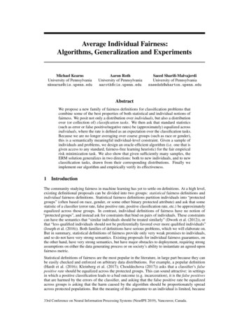
b (X, Wc ) – pseudocodeMapping 3: ψInput: f F (represented as {f (xi )}ni 1 )for t 1, . . . , T doc1i (wi,t 1/n)(1 f (xi )) for i [n].c0i (wi,t 1/n)f (xi ) for i [n].D {xi , c1i , c0i }ni 1 .hf,wt CSC (H; D)endPTOutput: ψbf T1 t 1 hf,wt (H)Figure 1: Illustration of generalization directions.Theorem 3.1 (In-sample Accuracy and Fairness). Suppose m0 O (log (nT /δ)/α2 ν 2 ). Let (bp, γb)be the output of Algorithm 2 and let (p, γ) be any feasible pair of variables for (2). We have that withb Q)b err (p; P,b Q)b 2ν, and that pb satisfies (3α, 0)-AIF with respectprobability 1 δ, err (bp; P,b Q).b In other words, for all i [n], E(xi , pb γb; Q)to the empirical distributions (P,b 3α.3.3Generalization theoremsWhen it comes to out-of-sample performance in our framework, unlike in usual learning settings,there are two distributions we need to reason about: the individual distribution P and the problemdistribution Q (see Figure 1 for a visual illustration of generalization directions in our framework).We need to argue that ψb induces a mapping that is accurate with respect to P and Q, and is fair foralmost every individual x P, where fairness is defined with respect to the true problem distributionQ. Given these two directions for generalization, we state our generalization guarantees in threesteps visualized by arrows in Figure 1. First, in Theorem 3.2, we fix the empirical distribution ofb and show that the output ψb of Algorithm 2 is accurate and fair with respect to thethe problems Qunderlying individual distribution P as long as n is sufficiently large. Second, in Theorem 3.3, we fixb and consider generalization along the underlying problemthe empirical distribution of individuals Pgenerating distribution Q. It will follow from the dynamics of the algorithm that the mapping ψbwill remain accurate and fair with respect to Q. We will eventually put these pieces together inTheorem 3.4 and argue that ψb is accurate and fair with respect to the underlying distributions (P, Q)simultaniously, given that both n and m are large enough. We will use OPT (see Definition 3.1) as ab See the supplementary file for detailed proofs.benchmark for the accuracy of the mapping ψ.b be the outputs of Algorithm 2 andTheorem 3.2 (Generalization over P). Let 0 δ 1. Let ψb and γe (m dH log (1/ν 2 δ))/α2 β 2 . We have that with probability 1 5δ, the mapping ψbsuppose n Ob Q) bb i.e., Px P ( E(x, ψ;b γ 5α) βsatisfies (5α, β)-AIF with respect to the distributions (P, Q),bbband that err (ψ; P, Q) OPT (α; P, Q) O (ν) O (αβ) .Theorem 3.3 (Generalization over Q). Let 0 δ 1. Let ψb and γb be the outputs of Algorithm 2 ande log (n) log (n/δ) /ν 4 α4 . We have that with probability 1 6δ, the mapping ψbsuppose m Ob Q) bb Q), i.e., P b ( E(x, ψ;satisfies (4α, 0)-AIF with respect to the distributions (P,γ 4α) 0x Pbbband that err (ψ; P, Q) OPT (α; P, Q) O (ν).bTheorem 3.4 (Simultaneous Generalization over P and Q). Let 0 δ 1. Letb ψ and γe (m dH log (1/ν 2 δ))/α2 β 2 and m be the outputs of Algorithm 2 and suppose n O e log (n) log (n/δ) /ν 4 α4 . We have that with probability 1 12δ, the mapping ψb satisfies (6α, 2β)Ob Q) γAIF with respect to the distributions (P, Q), i.e., Px P ( E(x, ψ;b 6α) 2β and thatberr (ψ; P, Q) OPT (α; P, Q) O (ν) O (αβ).Note that the bounds on n and m in Theorem 3.4 are mutually dependent: n must be linear in m, butm need only be logarithmic in n, and so both bounds can be simultaneously satisfied with samplecomplexity that is only polynomial in the parameters of the problem.7

4Experimental evaluationFigure 2: (a) Error-unfairness trajectory plots illustrating the convergence of algorithm AIF-Learn.(b) In-sample error-unfairness tradeoffs and individual errors for AIF-Learn vs. the baseline model:simple mixtures of the error-optimal model and random classification. Gray dots are shifted upwardsslightly to avoid occlusions.We have implemented the AIF-Learn algorithm and conclude with a brief experimental demonstration of its practical efficacy using the Communities and Crime dataset3 , which contains U.S. censusrecords with demographic information at the neighborhood level. To obtain a challenging instance ofour multi-problem framework, we treated each of the first n 200 neighborhoods as the “individuals”in our sample, and binarized versions of the first m 50 variables as distinct prediction problems.Another d 20 of the variables were used as features for learning. For the base learning oracleassumed by AIF-Learn, we used a linear threshold learning heuristic that has worked well in otheroracle-efficient reductions (Kearns et al. (2018)).Despite the absence of worst-case guarantees for the linear threshold heuristic, AIF-Learn seemsto empirically enjoy the strong convergence properties suggested by the theory. In Figure 2(a) weshow trajectory plots of the learned model’s error (x axis) versus its fairness violation (variation incross-problem individual error rates, y axis) over 1000 iterations of the algorithm for varying valuesof the allowed fairness violation 2α (dashed horizontal lines). In each case we see the trajectoryeventually converge to a point which saturates the fairness constraint with the optimal error.In Figure 2(b) we provide a more detailed view of the behavior and perfor

saeedsh@wharton.upenn.edu Abstract We propose a new family of fairness definitions for classification problems that combine some of the best properties of both statistical and individual notions of fairness. We posit not only a distribution over individuals, but also a distribution over (or collection of) classification tasks.