Transcription
Fine-Grained Urban Flow PredictionYuxuan Liang1 , Kun Ouyang1 , Junkai Sun3 , Yiwei Wang1 , Junbo Zhang3,4 , Yu Zheng3,4,5 ,David S. Rosenblum1,2 , Roger Zimmermann11 Schoolof Computing, National University of Singapore, Singaporeof Computer Science, George Mason University, VA, USA3 JD iCity, JD Technology, Beijing, China & JD Intelligent Cities Research, Beijing, China4 Artificial Intelligence Institute, Southwest Jiaotong University, Chengdu, China 5 Xidian University, Xi’an, ok.com2 DepartmentABSTRACT1INTRODUCTIONUrban flow prediction benefits smart cities in many aspects, such astraffic management and risk assessment. However, a critical prerequisite for these benefits is having fine-grained knowledge of the city.Thus, unlike previous works that are limited to coarse-grained data,we extend the horizon of urban flow prediction to fine granularitywhich raises specific challenges: 1) the predominance of inter-gridtransitions observed in fine-grained data makes it more complicatedto capture the spatial dependencies among grid cells at a globalscale; 2) it is very challenging to learn the impact of external factors(e.g., weather) on a large number of grid cells separately. To addressthese two challenges, we present a Spatio-Temporal Relation Network (STRN) to predict fine-grained urban flows. First, a backbonenetwork is used to learn high-level representations for each cell.Second, we present a Global Relation Module (GloNet) that captures global spatial dependencies much more efficiently comparedto existing methods. Third, we design a Meta Learner that takesexternal factors and land functions (e.g., POI density) as inputs toproduce meta knowledge and boost model performances. We conduct extensive experiments on two real-world datasets. The resultsshow that STRN reduces the errors by 7.1% to 11.5% compared tothe state-of-the-art method while using much fewer parameters.Moreover, a cloud-based system called UrbanFlow 3.0 has beendeployed to show the practicality of our approach.Accurately forecasting urban flows, such as predicting the totalcrowd flows entering and leaving each location (i.e., grid cell) ofa city during a given time interval [40, 41], plays an essential rolein smart city efforts. It can provide insights to the governmentfor decision making, risk assessment, and traffic management. Forexample, by foreseeing that an overwhelming crowd will streaminto a region ahead of time, the government can carry out trafficcontrol, send warnings or even evacuate people for public safety.One key property that must be considered in grid-based urbanflow prediction is spatio-temporal (ST) dependencies: the future of agrid cell is conditioned on its previous readings as well as neighbors’ histories. Moreover, urban flows are also impacted by externalfactors such as weather conditions and events. For example, heavysnow can sharply reduce traffic flows in many regions. To addressthese characteristics, many existing studies [6, 20, 36, 40–42] useconvolutional neural networks (CNNs) as the backbone structureto extract spatially near and distant dependencies; the temporal dependencies (e.g., at the recent, daily and weekly levels) are capturedusing different sub-branches. Meanwhile, the influence of externalfactors is encoded by some manually-designed subnetworks.16 hopsR164 hopsR2CCS CONCEPTS Information systems Spatial-temporal systems; Computing methodologies Artificial intelligence; Neural networks.Grid size: 600m 600mGrid size: 150m 150mKEYWORDSUrban flow prediction; spatio-temporal data; relational learning;convolution neural networks; urban computing.ACM Reference Format:Yuxuan Liang, Kun Ouyang, Junkai Sun, Yiwei Wang, Junbo Zhang, YuZheng, David S. Rosenblum and Roger Zimmermann. 2021. Fine-GrainedUrban Flow Prediction. In Proceedings of the Web Conference 2021 (WWW’21), April 19–23, 2021, Ljubljana, Slovenia. ACM, New York, NY, USA, 11pages. https://doi.org/10.1145/3442381.3449792This paper is published under the Creative Commons Attribution 4.0 International(CC-BY 4.0) license. Authors reserve their rights to disseminate the work on theirpersonal and corporate Web sites with the appropriate attribution.WWW ’21, April 19–23, 2021, Ljubljana, Slovenia 2021 IW3C2 (International World Wide Web Conference Committee), publishedunder Creative Commons CC-BY 4.0 License.ACM ISBN 42381.3449792Figure 1: Coarse-grained vs. fine-grained urban flows.In this paper, we focus on predicting urban flows at a fine-grainedlevel, which is important yet unexplored in the community. Finegrained flows can create exactness of the underlying dynamics ofthe city, encouraging better decision making. For instance, as shownin Figure 1, acquiring the traffic in a small area of interest with size150m 150m can help allocate police resources more precisely whileknowing that information at a district level with size 600m 600m isless useful. Notice that for a specific city, increasing the granularity(e.g., 600m 150m) is equivalent to obtaining higher resolution (e.g.,32 32 128 128). Thus, we use “high resolution” and “fine granularity” interchangeably. Although previous studies have shownpromising results at coarse-grained levels (e.g., 32 32 Beijing [40]),their architectures are not suitable for predicting fine-grained urbanflows due to the following specific challenges:
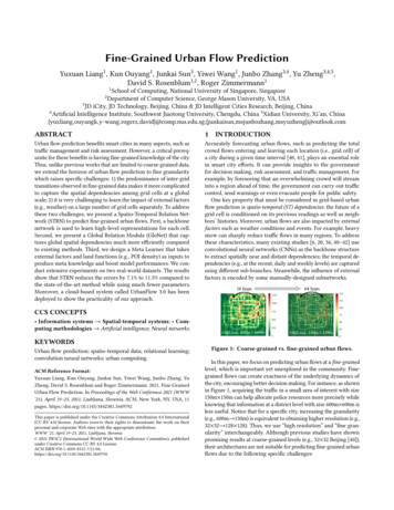
# of transitions (thousand)WWW ’21, April 19–23, 2021, Ljubljana, SloveniaingionRegionspaceCoarse-grained taxi flows (600m)240Fine-grained taxi flows (150m)160Time period:2013/07/01-2013/07/07800Gridspace# of hops14181121(a) An example of transitions0mLiang et al.(b) Space conversionFigure 2: (a) compares the transition patterns from a certainweek in Beijing. (b) shows grid- and region-based map segmentation, as well as space conversion between them.# of transitions (thousand)1) Global spatial dependencies. Rasterizing the city with higherresolution reveals more details of urban mobility and, meanwhile,enlarges the distance (or hops) between two given grid cells. Asshown in Figure 1(a), the number of hops between an office area(R1) and residence (R2) in Figure 1(b) becomes four times of thatin Figure 1(a). This causes the statistics in Figure 2(a) where wecan witness more long-range inter-grid communications (i.e., tranCoarse-grained taxi flows (600m)sitions with more hops) compared to that in the coarse-grained240Fine-grained taxi flows (150m)Regionsetting where short-range transitions oftenspacedominate. Hence, it160becomesfar more important to capture regional dependencies on aTime period:2013/07/01-2013/07/07global scale in such fine-grained settings. In most of the existing80studies [6, 40, 41], long-range spatial dependencies are capturedGrid# of hopsby large receptivefields achieved by stackingspace many convolutional014181121layers, where each layer captures only short-range dependencies(b) Transition during a time period in Beijing (c) From grid space to region spaceat a local scale. Such naive repetition is computationally inefficientand causes optimization difficulties [7]. Though using dilation convolution [39] tends to alleviate this drawback to some extent, it failsto improve the predictive performance empirically (see AppendixA for more details). These facts demonstrate that simply increasingthe receptive fields may not help. Recently, a new method calledDeepSTN [20] attempted to capture the global spatial dependencies in every layer by explicitly modeling all pairwise relationshipsbetween grids. However, it indispensably induces a huge number ofparameters with high computational costs. Hence, how to efficientlycapture the global spatial dependencies remains unsolved.2) External factors & Land functions. Previous studies like DeepST[41] and ST-ResNet [40] use subnetworks to map the effects of external factors onto each grid cell. Specifically, they stack severalfully-connected layers upon the external factors: the former layersact as embedding layers to combine each factor and the final layermaps the short embeddings to high-dimensional features with thesame shape as the flow map. However, as the resolution enhancesto a fine-grained level, it will induce a large number of parametersproportional to the number of grid cells in the final layer. Furthermore, they ignore the influence of land functions such as POIs ontraffic movements. To this end, DeepSTN [20] presents a new wayto jointly consider the POIs information as well as the externalfactors. However, in DeepSTN , external factors are used only tolearn the weights of different kinds of POI features, while ignoringthe significant difference of how external factors impact differentgrid cells. Thus, it is still challenging to learn the location-specificresponse to the external factors in fine-grained settings.To address the above challenges, we present a Spatio-TemporalRelation Network (STRN) for fine-grained urban flow prediction.Similar to the previous and current state-of-the-art methods [20, 40],STRN follows the CPT (closeness, period and trend) paradigm tomodel the three types of temporal dependencies, and uses a CNNbased backbone to extract high-level ST features. To address theabove challenges, we design two specific modules as follows.Primarily, we introduce a new structure (GloNet) to capture theglobal spatial dependencies. We partition a city into 𝑁 grid cells.Compared to DeepSTN that directly models all inter-grid correlations (totally 𝑁 2 correlations), we perform relational inferenceon a higher semantic level (i.e., region level) that is more friendlyto capture such global relations. As depicted in Figure 2(b), wefirst perform a conversion from grid space to region space (𝑀 regions), and then infer the regional correlations globally by messagepassing. Since the region semantic changes over time, a new lossbased on minimum cut theory enables the model to dynamicallypartition the map into irregular regions. Finally, we project thefeatures back to the grid space and obtain global-aware features. Inthis way, our method only needs to model 𝑀 2 correlations amongall region pairs1 , where typically 𝑀 𝑁 . Moreover, we presentan original Meta Learner to produce the cell-specific responses tothe time-evolving external factors based on matrix decomposition.Compared to DeepST and ST-ResNet, our Meta Learner not onlyconsiders the latent region functions but is also independent ofthe map resolution. Thus, it is more lightweight and practical infine-grained settings. In contrast to DeepSTN , our module cancapture the cell-specific responses to the external factors and learnbetter representations. In summary, our contributions are four-fold: We devise a unified model that jointly considers the spatial, temporal and external relations for predicting fine-grained urbanflows. A system has been deployed to show its practicality. We develop a GloNet structure that captures the global spatialdependencies in a more economical way than existing methods. We design an original Meta Learner to simultaneously learn theeffects of external factors and land function. We conduct extensive experiments to evaluate our model on tworeal-world mobility datasets. Our model reduces the errors by7.1% 11.5% while using as few as less than 1% of the number ofparameters required in the state-of-the-art method DeepSTN .2FORMULATIONDefinition 1 (Grid cell) As shown in Figure 3(a), we partition anarea of interest (e.g., a city) evenly into a 𝐻 𝑊 raster with totally𝑁 𝐻𝑊 grid cells. Note that enlarging 𝐻 or 𝑊 indicates that wecan obtain urban flow data with higher resolution.OfficeareaPartitionResidence(a) Map segmentation(b) Road network(c) Irregular regionsFigure 3: (a): Grid-based map segmentation. (b)-(c): We partition Beijing into irregular regions based on road networks.1For example, 𝑁 1282 16384 while 𝑀 100 in TaxiBJ dataset
Fine-Grained Urban Flow PredictiontimeexternalFetchExt & LandPOI&RNFeatures.tt-1t-221Label XtWWW ’21, April 19–23, 2021, Ljubljana, rendXqMetaLearnerConvConvConvLoss FunctionOmMincut lossMAE lossOcOp concatOq(1) Data loNet Prediction Xt(2) Model learning/predictingFigure 4: The framework of STRN. Closeness, period and trend are recent, daily and weekly patterns; Conv: convolution layer.Definition 2 (Urban flow) The urban flows at a certain time 𝑡 canbe denoted as a 3D tensor X𝑡 R𝐾 𝐻 𝑊 , where 𝐾 is the numberof flow measurements (e.g., inflow/outflow). Each entry (𝑘, ℎ, 𝑤)denotes the value of the 𝑘-th measurement in the cell (ℎ, 𝑤).Definition 3 (Region) Land use and function endow different geographic semantics to urban areas that are bounded irregularly [43].Figure 3(c) shows an example of irregular region segmentationbased on road networks. It provides us with a more natural andsemantic segmentation of urban spaces than the grid-based method.Assume that each region consists of many grid cells and we canthereby use a matrix B R𝑁 𝑀 to denote the assignment, whereeach element 𝑏𝑖,𝑗 is the likelihood that grid cell 𝑖 belongs to region𝑗 and 𝑀 is the number of regions.Definition 4 (External factors) Urban flow data have a strongcorrelation with external factors, such as weather conditions, timeof day and events. We denote these external factors at a certaintime step 𝑡 as a vector e𝑡 R𝑙𝑒 , where 𝑙𝑒 is the feature length.Definition 5 (Land features) The category of POIs and their density in an urban grid cell indicate the land functions of the cell aswell as the traffic patterns in this cell, therefore contributing to theurban flows of the grid cell [20]. Likewise, the structure of roadnetworks (RNs) like the number of high-level road segments alsoprovides a good complement to traffic modeling [17, 43]. Thus, wecombine the land features including POIs and RNs of every cell,and denote them as P R𝑙 𝑓 𝐻 𝑊 , where 𝑙 𝑓 is the feature number.Problem Statement Here, we define the problem of fine-grainedurban flow prediction: Given the fine-grained historical observations of urban flows denoted as {X𝑖 𝑖 1, 2, · · · , 𝑡 1}, the corresponding external factors e𝑡 , and the land features P, our target isto predict the urban flows at the future time step, denoted as X𝑡 .3METHODOLOGYFigure 4 illustrates the framework of STRN, which consists of twomajor stages: data preparation and model learning/predicting. Inthe first stage, we first select the key timesteps (closeness, periodand trend) to create the flow inputs, denoted as X𝑐 , X𝑝 and X𝑞 ,respectively. Meanwhile, we fetch the context of the external factorse𝑡 and the land features P. More details about the construction anddimensionality of these inputs are provided in Appendix B.In the second stage, the prepared data are fed to learn the model,following a local to global paradigm. As shown in Figure 4, for eachtemporal sequence (X𝑐 , X𝑝 and X𝑞 ), we first use three non-sharedconvolutional layers to convert them to embeddings O𝑐 , O𝑝 , O𝑞 ,each with 𝐷 channels, i.e., they are all in R𝐷 𝐻 𝑊 . Meanwhile,we design a Meta Learner that takes the external factors and landfeatures as inputs to learn the external impacts on each urban gridcell, where the learned representation O𝑚 is of the same shape asO𝑐 . Next, we concatenate the three types of temporal features aswell as the meta features, and feed the fusion result O R4𝐷 𝐻 𝑊to the backbone network for feature extraction within its local receptive fields. This early fusion strategy allows different kinds ofinformation to interact with each other in the backbone network.Once we obtain the extracted high-level features Xℎ R𝐶 𝐻 𝑊at a local scale, we design a GloNet structure to capture the globalspatial dependencies and generate the final predictions. Finally,we optimize the model weights by using a loss function includingtwo parts: a Mincut loss for automatic region partition and a meanabsolute error (MAE) loss for measuring the prediction errors.3.1Backbone NetworkA powerful backbone network is crucial to urban flow predictionas it can help the model learn useful and discriminative features.For example, DeepST [41] provides the first deep learning-basedsolution to urban flow prediction by stacking a number of convolutional blocks for spatio-temporal feature extraction. As the networkdepth increases, DeepST will be hard to train due to the notoriousvanishing gradient problem. To overcome this drawback, ResNet[7] is widely used as the backbone in the previous and currentstate-of-the-art [6, 20, 40] for urban flow prediction. However, theyemphasize the dependencies in the spatial dimension and overlookthe channel-wise information in the feature maps. In this paper,we employ the Squeeze-and-Excitation Networks (SENet) [10] tofuse both spatial and channel-wise information within small (i.e.,local) receptive fields at each layer, which has proven to be effectivein producing compacted and discriminative features of each gridcell. As shown in Figure 4, it takes the fusion result O as input andoutputs the high-level representations of each cell. First, we use aconvolutional layer to compress the dimension of input channelsfrom 4𝐷 to 𝐶. Then, we stack 𝐹 squeeze-and-excitation (SE) blocks[10] with 𝐶 filters for feature extraction within the receptive field.Finally, a convolution layer is used to generate the output Xℎ . Thevisualization of pipeline can be found in Appendix C.
WWW ’21, April 19–23, 2021, Ljubljana, SloveniaLiang et al.Grid FeaturesH: M C’MessagePassing(GCN)Region FeaturesReverseProjectionReshape&Predict Ar:Xt : K H WSpaceConversionXg : N CRegion BPartitionH’ : M C’Xh : N CRegion spaceRegion FeaturesGrid FeaturesPredictionsFigure 5: The pipeline of GloNet, where 𝑁 𝐻𝑊 and 𝑀 are the number of grid cells and regions respectively.3.2Global Relation Moduleaim to generate the grid-to-region assignment matrix B R𝑁 𝑀 ,where 𝑀 is a hyperparameter that indicates the number of regions.Although we can perform a static region segmentation based onthe road networks as mentioned in Section 2, it fails to capture thehighly dynamic traffic conditions and the time-evolving externalfactors. To tackle this problem, we compute B based on the highlevel representation Xℎ by means of a function 𝛿, which maps eachgrid feature xℎ𝑖 into the 𝑖-th row of B as B softmax 𝛿 (Xℎ ) ,(1)where the softmax function guarantees the sum of each columnequals to one. We parametrize 𝛿 as a feedforward neural network.Inspired by the Mincut theory [1, 30] that aims at partitioningnodes into disjoint subsets by removing the minimum volume ofedges, we view each region as a cluster containing many grid cellsand regularize the assignment matrix by using a new loss. In otherwords, the network weights can be jointly optimized by minimizingthe usual task-specific loss (e.g., MAE loss), as well as an unsupervised Mincut loss L𝑚 composed of two terms:Y: K H WXg: N CH’ : M C’Xh: N CB𝑇 BITr(B𝑇 Ã𝑔 B)After local feature extraction, we present a Global Relation Mod 𝑀 ,(2)L𝑚 ule (GloNet) to capture the global spatial dependencies in a moreB𝑇 B 𝐹Tr(B𝑇 D̃𝑔 B)𝑀 𝐹 {z} {z}economical way than the previous attempts (e.g., DeepSTN ). MotiRegion spaceL𝑐L𝑜vated by the relation networks [2, 14, 44] seizing relations betweenwhere · 𝐹 denotes the Frobenius norm; Tr is the trace of a matrix;objects in images, we perform relationalinference on a higher seA:reshapeSpaceMessage𝑁 𝑁 is the adjacency matrixA𝑔 RRederivedConv from the Euclideanmantic level (i.e., region level) that is more friendly to capture globalConversionPassingprojection 𝑔𝑔 is the degree matrix ofstructureandÃisitsnormalization;D̃relations. Moreover, we design an unsupervisedlossbasedontheH: M C’𝑔𝑇Ã . I𝑀 B̂ B̂ is a rescaled clustering matrix, where B̂ assignsminimum cut (Mincut) theory for region partition.exactly 𝑁 /𝑀 gridcells to each region. L𝑐 [ 1,0] denotes theFigure5 depicts the whole pipelineGloNet. We first use Regionthe FeaturesGrid FeaturesRegionofFeaturesGrid FeaturesPredictionsconsistency loss that evaluates the mincut given by B. Minimizinghigh-level features Xℎ to generate the assignment matrix B by aL𝑐 enforces strongly connected grid cells to be grouped into thelinear transformation. By referring to this matrix, GloNet then agsame region, while the other term L𝑜 encourages the assignmentgregates the grid-cell features into region space to obtain region′to be orthogonal and the regions to be of similar size (see proof infeatures H R𝑀 𝐶 and generate the connections (i.e., adjacencyAppendix D). Since the two terms in L𝑜 have unitary norm, it ismatrix A𝑟 R𝑀 𝑀 ) between these regions. As the regions areTobvious that 0 L𝑜 2. Hence, L𝑜 does not dominate over L𝑐 .connected in the form of a graph, we utilizeConvolutionBGraphNetworks (GCN) [13] to perform message passing on the region3.2.2 Space Conversion. Given the grid-cell features and the aslevel. Once we obtain the global-aware features that are discrimisignment matrix, we convert those grid-based embeddings to their′native on the region level, the last step of GloNet is to project themregional counterparts H R𝑀 𝐶 that are more friendly to captureback to the grid space and generate the finalBpredictions.global dependencies. Moreover, we need to find the connectivityA𝑟 R𝑀 𝑀 between these regions. As people are capable of travel3.2.1 Region Partition. Recall that the backbone network has proing to remote places in a short time period (e.g., 30 minutes) in modduced a high-level abstraction of the flow history and external conern cities, we assume that all regions are mutually connected (i.e., atexts. For convenience, we reshape this tensor to be Xℎ R𝑁 𝐶 ,complete digraph). Instead of using complex and time-consumingwhere 𝑁 𝐻𝑊 is the number of grid cells. By doing this, eachoperations, we implement the space conversion bygrid 𝑖 can be represented by an embedding xℎ𝑖 R𝐶 . Here, weH B 𝜙 (Xℎ ),A𝑟 B Ã𝑔 B,(3)where we generate the features of each region by directly aggregating the features of the corresponding cells that belong to this region;𝜙 is a dense layer that compresses the dimension of embeddingsfrom 𝐶 to 𝐶 ′ to avoid heavy computation; A𝑟 is a symmetric matrix,whose entry 𝑎𝑖,𝑖 is the total number of edges between the grid cellsin the region 𝑖, while 𝑎𝑖,𝑗 is the number of edges between region 𝑖and 𝑗. It can be seen easily that A𝑟 comes from the numerator of𝐿𝑐 in Eq. 2, thus, the trace maximization yields regions with manyinternal grid-cell connections and weakly connected to each other.3.2.3 Message Passing between Regions. After space conversion,we obtain a new graph where each node represents an irregularregion and each edge models the interaction among two regions. Tomodel the inter-region relationships, a natural idea is to use GraphConvolutional Networks (GCN) [13] to perform message passingbetween these regions based on A𝑟 . However, we notice that A𝑟is a diagonal-dominant matrix, describing a graph with self-loopsmuch stronger than any other connection. As self-loops usuallyhamper the propagation across adjacent nodes in message passing
(a) Food & BeverageFine-Grained Urban Flow Predictionwhere D̂ denotes the degree matrix of Â𝑟 . Then, we employ a twolayer GCN for global relation inference on the region graph to′generate the new region features H ′ R𝑀 𝐶 as H ′ 𝑓𝐺𝐶𝑁 ( Ã𝑟 , H) Ã𝑟 ReLU Ã𝑟 HW1 W2(5)lfNPOIs & RNsLand FeaturesLOmNGrid-cellEmbeddings2-layerMLPExternal FactorsDMatmulreshapeOutputreshapeExternal FeatureslfRParameterEmbeddingsDFigure 6: Pipeline of the proposed Meta Learner.′where W1, W2 R𝐶 𝐶 are learnable weights. By this, the regionalinformation are passed through the graph to generate a globalaware representation for each region.3.2.4 Reverse projection. Once we obtain the global-aware featuresH ′ from region space, the next step is to project them back to theoriginal space. Similar to the step of space conversion, we can alsouse an assignment matrix for the reverse projection. Instead ofusing extra operations and introducing additional overhead, wereuse the B R𝑁 𝑀 to project the region features back to grid-cellfeatures by a linear combination as follows:𝑔′X B𝜃 (H ),(6)where 𝜃 is a dense layer for dimension conversion from 𝐶 ′ to 𝐶. Thenew grid-cell features X𝑔 R𝑁 𝐶 are generated by aggregatingtheir related region features, which is achieved by multiplyingmatrix 𝜃 (H ′ ). Until now, we have performed a grid-region-gridtransformation to learn the global-aware features in this module.3.2.5 Reshape & Predict. Lastly, the global-aware discriminativefeatures X𝑔 are reshaped to R𝐶 𝐻 𝑊 such that the output dimension can match the input dimension Xℎ forming a residual path,and fed to a convolution layer to produce the final predictions X̂𝑡 .In practice, the matrix multiplication procedures for projection andreverse projection are both implemented by an 1 1 convolutionlayer since it supports high-speed parallelization. When computingthe Mincut loss, we need to store and employ two matrices (i.e.,Ã𝑔 and D̃𝑔 ) with shape 𝑁 by 𝑁 , which dramatically increases thememory cost and computational cost in devices (such as a GPU).To overcome this problem, we notice these two matrices are sparseand thereby implement Eq. 2 based on sparse matrix multiplication.3.3(c) level-2 roadsWWW ’21, April 19–23, 2021, Ljubljana, Sloveniaschemes [13], we compute a new adjacency matrix Ã𝑟 R𝑀 𝑀 byzeroing the diagonal and applying degree normalization: 11(4)Â𝑟 A𝑟 diag A𝑟 ; Ã𝑟 D̂ 2 Â𝑟 D̂ 2′(b) level-1 roadsMeta LearnerAs mentioned before, existing works like DeepST [41] and STResNet [40] use fully-connected layers to encode the external factors for urban flow prediction. However, as the granularity becomeslarger to a fine-grained setting, it will induce massive parametersin the last layer proportional to the number of grid cells (𝑁 ). Inaddition, they do not consider the influence of land features onthe traffic movements. To this end, DeepSTN [20] presents a newapproach to jointly consider the POIs information as well as theexternal factors. They notice that POIs have varied temporal influences on flow maps, they thereby transform the external factors toinfluence the strength of POI. However, the external factors are applied to weight on different channels (i.e., categories) of POIs whileignoring the significant difference of how external factors impactdifferent cells. Thus, how to learn the cell-specific responses to theexternal factors in the fine-grained settings remains a challenge.In general, grid cells with similar land functions will have similarresponses to the external factors. Based on this observation, wedesign a novel Meta Learner to produce cell-specific responses tothe external factors based on Matrix Factorization. Given the landfeatures P R𝑙 𝑓 𝐻 𝑊 and external features e𝑡 R𝑙𝑒 , we aim tocompute the response of each grid cell byO𝑚 𝑓𝑀𝐿 (P, e𝑡 ) R𝐷 𝐻 𝑊 .(7)Then, the output O𝑚 will be early fused with the temporal information (O𝑐 , O𝑝 , O𝑞 ) and fed to the backbone network.Without introducing a large number of parameters in 𝑓𝑀𝐿 , wecan reshape this target tensor as R𝑁 𝐷 and decompose it intotwo matrices L R𝑁 𝑘 and R R𝑘 𝐷 , which satisfies O𝑚 LR.Motivated by a very recent study that learns specific predictors foreach grid cell [27], we can view L as the grid-cell embeddings whileR represents the parameter embeddings generated using e𝑡 as metaknowledge. For simplicity, L is reshaped from the land featuresP, where 𝑙 𝑓 𝑘 at this time. In this way, we can guarantee thatcells with similar land functions will have similar responses to theexternal factors. For the parameter embeddings R, we aim to makeit change over time and influenced by the external factors, suchas weather and time. Inspired by the meta learning approach fortraffic prediction [27], we can use a two-layer MLP to generate it:the first layer transforms the external features from 𝑙𝑒 to 𝑙𝑑 , andthe second layer further converts the dimension to be 𝑙 𝑓 𝐷. Finally,we reshape the output and assign it to R.To help better understand the meta learner, Figure 6 furtherdescribes its whole pipeline. Compared to external components inST-ResNet, as our meta learner is independent of the map resolution(only 𝑙𝑒 𝑙𝑑 𝑙𝑑 𝑙 𝑓 𝐷 parameters, which can be set far less than 𝑁 ),it is much more lightweight and practical in fine-grained settings.In contrast to DeepSTN , our module can capture the cell-specificresponses to the external factors and learn better representations.3.4OptimizationOur method provides an end-to-end solution from historical observations to fine-grained predictions, which is differentiable everywhere. Hence, the network can be trained through the backpropagation strategy and the Adam optimizer. To train our model,we aim to minimize the following loss function with two terms:L L𝑀𝐴𝐸 𝛼 L𝑚 .(8)Here, 𝛼 is a trade-off between these two losses while L𝑀𝐴𝐸 is thepixel-wise Mean Absolute Error (MAE) for evaluating the errorsb𝑡 and the corresponding ground truth X𝑡 .between our prediction X
WWW ’21, April 19–23, 2021, Ljubljana, SloveniaLiang et al.4 EVALUATION4.1 Experimental Settings4.1.1 Datasets. We conduct our experiments on two real-worlddatasets, where TaxiBJ is the fine-grained version of TaxiBJ released by [41] and HappyValley is from [19]. TaxiBJ : This dataset sources from the trajectories of over 30,000taxicabs in Beijing for four different time periods (i.e., P1 to P4).Since the taxi distributions and numbers are different in thesefour time periods, we evaluate our method over these periodsseparately. As shown in Figure 1(b), we crop the area of interestwhich contains most traffics, and rasterize this area into 128 128uniform grid cells. The size of each cell is 150m 150m, which
uisite for these benefits is having fine-grained knowledge of the city. Thus, unlike previous works that are limited to coarse-grained data, we extend the horizon of urban flow prediction to fine granularity which raises specific challenges: 1) the predominance of inter-grid transitions observed in fine-grained data makes it more complicated