Transcription
powered byMODELING IN XCOS USING MODELICAIn this tutorial we show how to model a physical system described by ODE usingthe Modelica extensions of the Xcos environment. The same model has beensolved also with Scilab and Xcos in two previous tutorials.LevelThis work is licensed under a Creative Commons Attribution-NonCommercial-NoDerivs 3.0 Unported License.www.openeering.com
Step 1: The purpose of this tutorialScilab provides three different approaches (see figure) for modeling aphysical system described by Ordinary Differential Equations (ODE).For showing all these capabilities we selected a common physicalsystem, the LHY model for drug abuse. This model is used in ourtutorials as a common problem to show the main features for eachstrategy. We are going to recurrently refer to this problem to allow thereader to better focus on the Scilab approach rather than on mathematicaldetails.In this third tutorial we show, step by step, how the LHY model problemcan be implemented in the Xcos Modelica environment. The samplecode can be downloaded from the Openeering web site.1Standard ScilabProgramming2Xcos Programming3Xcos ModelicaStep 2: Model descriptionThe considered model is the LHY model used in the study of drug abuse.This model is a continuous-time dynamical system of drug demand for twodifferent classes of users: light users (denoted by) and heavy users(denoted by) which are functions of time . There is another state inthe model that represents the decaying memory of heavy users in theyears (denoted by) that acts as a deterrent for new light users. Inother words the increase of the deterrent power of memory of drug abusereduces the contagious aspect of initiation. This approach presents apositive feedback which corresponds to the fact that light users promoteinitiation of new users and, moreover, it presents a negative feedbackwhich corresponds to the fact that heavy users have a negative impact oninitiation. Light users become heavy users at the rate of escalation andleave this state at the rate of desistance . The heavy users leave thisstate at the rate of desistance .Tutorial Xcos Modelicawww.openeering.compage 2/19
Step 3: Mathematical modelThe mathematical model is a system of ODE (Ordinary DifferentialEquation) in the unknowns: , number of light users; , number of heavy users; , decaying of heavy user years.The LHY equations system (omitting time variable for sake of simplicity) iṡ{ ̇̇where the initiation function isThe initiation function contains a “spontaneous” initiationand amemory effect modeled with a negative exponential as a function of thememory of year of drug abuse relative to the number of current light users.{}The LHY initial conditions areThe problem is completed with the specification of the initial conditionsat the time .{Tutorial Xcos Modelicawww.openeering.compage 3/19
Step 4: Problem dataModel data(Model data): the annual rate at which light users quit: the annual rate at which light users escalate to heavy use: the annual rate at which heavy users quit: the forgetting rateInitiation function(Initiation function): the number of innovators per year: the annual rate at which light users attract non-users: the constant which measures the deterrent effect of heavy use: the maximum rate of generation for initiation(Initial conditions)Initial conditions: the initial simulation time;: Light users at the initial time;: Heavy users at the initial time;: Decaying heavy users at the initial time.Tutorial Xcos Modelicawww.openeering.compage 4/19
Step 5: Xcos Modelica programming – introductionModelica is a component-oriented declarative language useful formodeling the behavior of physical systems, consisting of electrical,hydraulic, mechanical and other domains.Modelica language is useful for exchanging mathematical models since itprovides a way to describe model components and their structure inlibraries. The description of the these models is done using a declarativelanguage based on equations, in contrast to usual programming that isbased on the use of assignment statements. This permits a great flexibilityand enhance reading scheme since equations have no pre-definedcausality, equations do not have a pre-defined input/output relation,models are acausal models.Modelica blocks are identical to standard Xcos blocks except for the factthat are of implicit type. Blocks with implicit dynamic ports mean that theconnections between two or more ports do not impose any transfer ofinformation in a known direction. These blocks are denoted by a blacksquare and the user can connect implicit blocks of the same domain.Modelica blocks in Xcos require a C compiler since Modelica translatesthe system directly into a C file that is then linked to the Xcosenvironment. To check if a compiler is available in your Scilabenvironment use command “haveacompiler”. For information aboutsupported and compatible compilers see Scilab documentation.In the figure we show the available blocks for the “Electrical” palette.Tutorial Xcos Modelicawww.openeering.compage 5/19
Step 6: Across and ThroughAn import concept to understand how Modelica block work is thedifference between “across” and “through” variables: “Across”: A variable whose value is determined by the measurewith an instrument in parallel;(e.g. voltage for the electrical domain) “Through”: A variable whose value is determined by the measurewith an instrument in series.(e.g. current for the electrical domain)Typically, the product of an across variable with a through variable is thepower exchanged by the element.Step 7: RoadmapIn this tutorial we describe how to construct the LHY model and how tosimulate it in Xcos Modelica. We implement the system in the followingway: First we provide a comparative example (RLC circuit) betweenXcos and Modelica; A general description of the “Modelica Blocks” available in Xcos isgiven; Then we implement the LHY model in Xcos Modelica; In the end, we test the program and visualize the results.Tutorial Xcos Modelicawww.openeering.comDescriptionsRLC – exampleXcos MBLOCKLHY exampleTest and visualizeSteps8-1112-1617-2021page 6/19
Step 8: RLC ExampleA comparative example, based on a RLC electric circuit, is use to showthe differences between a pure Xcos diagram and an Xcos Modelicascheme.The adopted scheme, reported on the right, is composed of the followingcomponents: Voltage source (Amplitude A 2.0 [V], Frequency f 1 [Hz]); with equation:; Resistor (Resistance; Inductor (Inductance L 0.0001 [H], Initial current 0) with equation: Capacitor (Capacitance C 0.1 [F], Initial voltage 0) with equation:R 0.2[Ohm]) with equation:where we are interested in measuring the voltage across the capacitorand the current through the voltage source.Tutorial Xcos Modelicawww.openeering.compage 7/19
Analytical solution:Step 9: RLC – Analytical solutionIf we write the equation for the 8 unknowns variablesandwe have:,,(2 equations)(Kirchhoff’s current law)((2 equations))(Kirchhoff’s voltage law)(4 equations)(Constitutive equations)which have the following analytical solution:The analytical solution is plotted on the right:andTutorial Xcos Modelica.www.openeering.compage 8/19
Step 10: RLC Xcos model1There are many Xcos blocks formulation for the RLC circuit but onewhich allows fast and accurate results is the one that uses only integrationblocks instead of derivate blocks.Hence, the idea is to start from the equalityfollowing part of the scheme:and make theThe next step is to add “sum blocks” that represent the local conversion ofKirchhoff’s laws:and to add the model of1as follows:See “Introduction to Control Systems in Scilab”, Scilab Tutorials, Openeering, 2012Tutorial Xcos Modelicawww.openeering.compage 9/19
Step 11: RLC with Xcos ModelicaHere, we use elements available in the “Electrical” Palette to make thesystem.First of all, it is necessary to note that at each node there are the localconservation of the through (or flux) variable “current” and of the acrossvariable “potential”.The following elements are used: Ground that fixes the reference potential; AC voltage source that is the active element of the network; Resistor, Inductor and Capacitor that are the passive elements ofthe networks; Voltage and Current sensors that are used as interface elements(data exchange) from Modelica to Xcos.Tutorial Xcos Modelicawww.openeering.compage 10/19
The Modelica generic blockStep 12: Basic Modelica blocks – The MBLOCKPalette: User defined functions / MBLOCKPurpose: This block provides an easy way for creating an Xcos interfacefor Modelica without creating any interfacing functions.Step 13: Dialog box of the MBLOCK (input/output)The MBLOCK dialog interfaceIn order to construct an Xcos/Modelica block it is necessary to specify thefollowing: Input variables: name of input ports. Remember that two types ofports are available:-Explicit: In this case, variables should be declared in theModelica program as Real);Implicit: In this case, variables should be connectors. Input variables types: In this field, the type of input ports isspecified. Two options are available:E: for explicit ports;I: for implicit ports. Output variables: Similar to input variables settings; Output variables types: Similar to input variables types;Tutorial Xcos Modelicawww.openeering.compage 11/19
Step 14: The dialog box of the MBLOCK (parameters)In order to construct an Xcos/Modelica block it is necessary to specify thefollowing information: Parameters in Modelica: model parameters that are initialized ina second dialog box; Parameters properties: The type of the Modelica parameters:0: for a Modelica parameter variable (scalar or vector);1: for an initial condition of Modelica state variable (scalaror vector);2: for an initial condition of Modelica state variable withthe property fixed true (scalar or vector). Function name: The name of the Modelica class without anyspecification of paths or extensions. The Modelica classassociated to this block can be either given in a file or specified inthe dialog of the block. If the Modelica class name is specifiedwith its path and the “.mo” extension, the compiler looks for thefile and if it is found, the file will be compiled. If the file is notspecified or is not found, a window is opened and the user canedit the Modelica program.Tutorial Xcos Modelicawww.openeering.comThe MBLOCK dialog interfacepage 12/19
Step 15: Example of MBLOCK for RLC circuitThe aim of the following example is to develop a new element forcomputing the instantaneous electric powerdelivered by aresistive element.The idea is to re-write the “model Resistor” such that it provides a furtheroutput that contains its instantaneous power. In this case we use thefollowing external model file (“PowerResistor.mo”):model PowerResistor// Define input/output model port// Pin p, n;extends TwoPin;// Model paramterparameter Real R 1 "Resistance";// Output power portReal PVal;equationPVal v*i;R*i v;end PowerResistor;Tutorial Xcos Modelicawww.openeering.compage 13/19
16: Example of MBLOCK for RLC circuitThe interface using MBLOCK is defined as follows: Input variables: "p" Input variables types: "I" Output variables: ["n";"PVal"] Output variables types: ["I";"E"] Parameters in Modelica: ["R"] Parameters properties: [0] Function name: PowerResistor.moThe simulation output is reported on the right.Tutorial Xcos Modelicawww.openeering.compage 14/19
Step 17: Create a LHY block – step 1The first step is to specify the interface as follows: Input variables: (empty) Input variables types: (empty) Output variables: ["Ival";"Lval";"Hval";"Yval"] Output variables types: ["E";"E";"E";"E"] Parameters in ;"L";"H";"Y"] Parameters properties: [0;0;0;0;0;0;0;0;1;1;1] Function name: lhymodelStep 18: Create a LHY block – step 2The next step is to specify the value of the model parameters as reportedin the problem data slide.Tutorial Xcos Modelicawww.openeering.compage 15/19
Step 19: Create a LHY block – step 3Write the Modelica lhymodel class.class lhymodel////automatically generated //////parametersparameter Real tau 5.000000e 004;parameter Real s 6.100000e-001;parameter Real smax 1.000000e-001;parameter Real q 3.443000e 000;parameter Real a 1.630000e-001;parameter Real b 2.400000e-002;parameter Real g 6.200000e-002;parameter Real delta 2.910000e-001;RealL (start 1.400000e 006);RealH (start 1.300000e 005);RealY (start 1.100000e 005);//output variablesReal Ival,Lval,Hval,Yval;////do not modify above this line ////equation// OutputLval L;Hval H;Yval Y;// Initiation equationIval tau max(smax,s*exp(-q*Y/L))*L;// LHY modelder(L) Ival - (a b)*L;der(H) b*L - g*H;der(Y) H - delta*Y;end lhymodel;Tutorial Xcos Modelicawww.openeering.compage 16/19
Step 20: Create a LHY schemeComplete the scheme adding a multiplexer block, a scope block and aclock block.Step 21: Running and testingRun and test the example.Tutorial Xcos Modelicawww.openeering.compage 17/19
Step 22: Exercise #1Modify the main program file such that it is possible to have the LHY withdifferent values for parameter (e.g. the original value and its double).Compare the results in a unique plot where all the , , and have thesame color.Step 23: Concluding remarks and References1. Scilab Web Page: Available: www.scilab.org.In this tutorial we have shown how the LHY model can be implemented inScilab/Xcos Modelica2. Openeering: www.openeering.com.On the right-hand column you may find a list of references for furtherstudies.3. D. Winkler, J. P. Caulkins, D. A. Behrens and G. Tragler, "Estimatingthe relative efficiency of various forms of prevention at differentstages of a drug epidemic," Heinz Research, orial Xcos Modelicawww.openeering.compage 18/19
Step 24: Software contentTo report a bug or suggest some improvement please contact Openeeringteam at the web site www.openeering.com.Thank you for your attention,Manolo VenturinTutorial Xcos Modelica--------------------------------LHY MODEL IN ---------------Main directory-------------ex1.xcos: Solution of the exerciseLHY Tutorial Xcos Modelica.xcos: Main programlicense.txt: The license filePowerResistor.mo: PowerResistor modelRLC Analytical.sce: RLC analytical solution plotRLC Power.xcos: RLC with PowerResistor elementRLC Xcos.xcos: RLC in xcosRLC Xcos Modelica.xcos: RLC in xcos/Modelicawww.openeering.compage 19/19
Tutorial Xcos Modelica www.openeering.com page 3/19 Step 3: Mathematical model The mathematical model is a system of ODE (Ordinary Differential Equation) in the unknowns: , number of light users; ,number of heavy users; , decaying of heavy user years. The initiation function contains a "spontaneous" initiation and a