Transcription
powered byMODELING IN SCILAB: PAY ATTENTION TO THE RIGHTAPPROACH – PART 1In this tutorial we show how to model a physical system described by ODE usingScilab standard programming language. The same model solution is alsodescribed in Xcos and Xcos Modelica in two other tutorials.LevelThis work is licensed under a Creative Commons AttributionAttribution-NonCommercial-NoDerivs 3.0 Unported License.www.openeering.com
Step 1: The purpose of this tutorialIn Scilab there are three different approaches (see figure) for modelinga physical system which are described by Ordinary Differential Equations(ODE).For showing all these capabilities we selected a common physicalsystem, the LHY model for drug abuse. This model is used in ourtutorials as a common problem to show the main features of eachstrategy. We are going to recurrently refer to this problem to allow thereader to better focus on the Scilab approach rather than on mathematicaldetails.1Standard ScilabProgramming2Xcos Programming3Xcos ModelicaIn this first tutorial we show, step by step, how the LHY model problemcan be implemented in Scilab using standard Scilab programming. Thesample code can be downloaded from the Openeering web site.Step 2: Model descriptionThe considered model is the LHY model used in the study of drug abuse.This model is a continuous-time dynamical system of drug demand for twodifferent classes of users: light users (denoted by) and heavy users(denoted by) which are functions of time . There is another state inthe model that represents the decaying memory of heavy users in the) that acts as a deterrent for new light users. Inyears (denoted byother words the increase of the deterrent power of memory of drug abusereduces the contagious aspect of initiation. This approach presents apositive feedback which corresponds to the fact that light users promoteinitiation of new users and, moreover, it presents a negative feedbackwhich corresponds to the fact that heavy users have a negative impact oninitiation. Light users become heavy users at the rate of escalationand leave this state at the rate of desistance . The heavy users leavethis state at the rate of desistance .LHY Tutorial Scilabwww.openeering.compage 2/12
Step 3: Mathematical modelThe mathematical model is a system of ODE (Ordinary DifferentialEquation) in the unknowns: L t , number of light users;The LHY equations system (omitting time variable t for sake of simplicity) isLHYH t , number of heavy users;Y t , decaying of heavy user years.I L, YabL gHH δYb Lwhere the initiation function isThe initiation function contains a “spontaneous” initiation τ and amemory effect modeled with a negative exponential as a function of thememory of year of drug abuse relative to the number of current light users.I L, Y)τL max s"# , s · e'(* The LHY initial conditions areThe problem is completed with the specification of the initial conditionsat the time t .LHY Tutorial Scilabwww.openeering.comL tH tY tLHYpage 3/12
Step 4: Problem dataModel data(Model data)a : the annual rate at which light users quitb : the annual rate at which light users escalate to heavy use0.163g0.062bg : the annual rate at which heavy users quitδ : the forgetting rateδ0.0240.291Initiation function(Initiation function)τ : the number of innovators per yearτs : the annual rate at which light users attract non-userssq : the constant which measures the deterrent effect of heavy useqs"# : the maximum rate of generation for initiation500000.610s"# (Initial conditions)3.4430.1Initial conditionst : the initial simulation time;tL : Light users at the initial time;LH : Heavy users at the initial time;HY : Decaying heavy users at the initial time.LHY Tutorial ScilabaYwww.openeering.com19701.4 7 1080.13 7 1080.11 7 108page 4/12
Step 5: Scilab programmingWith the standard approach, we solve the problem using the ODE functionavailable in Scilab. This command solves ordinary differential equationswith the syntax described in the right-hand column.In our problem we have: Y0 equal toY ;9 ,,: since the unknowns areThe syntax of the ode function isy ode(y0,t0,t,f)where at least the following four arguments are required:,andt0 equal to 1970;t generated using the command Y0 : the initial conditions [vector] (the vector length should beequal to the problem dimension and its values must be in the sameorder of the equations. t0 : the initial time [scalar] (it is the value where the initialconditions are evaluated); t : the times steps at which the solution is computed [vector](Typically it is obtained using the function LINSPACE or using thecolon : operator); f : the right-hand side of system to be solved [function,external, string or list].t Tbegin:Tstep:(Tend 100*%eps);which generates a regularly spaced vector starting from Tbeginand ending at Tend with a time-step Tstep. A tolerance is addedto ensure that the value Tend is reached. See also linspacecommand for an alternative solution. f a function of three equations in three unknowns whichrepresents the system to be solved.LHY Tutorial Scilabwww.openeering.compage 5/12
Step 6: RoadmapWe implement the system in the following way: Create a directory where we save the model and its supportingfunctions. The directory contains the following files:-A function that implements the initiation function;A function that implements the system to be solved;A function that plots the results. Create a main program that solves the problem; Test the program and visualize the results. LHY Initiation.sci: The initiation function LHY System.sci: The system function LHY Plot.sci: The plotting function LHY MainConsole.sce: The main function.Step 7: Create a working directoryWe create a directory, name it "model" in the current working folder(LHYmodel) as shown in figure.LHY Tutorial Scilabwww.openeering.compage 6/12
Step 8: Create the initiation functionNow, we implement the following formula; ,as a Scilab function. max "# , · '?@A The function returns the number of initiated individuals ; per years usingthe current value of , and its parameters , , B, "# . We decide toimplement the function parameters as a Scilab mlist data structure.The following code is saved in the file "LHY Initiation.sci" in themodel directory.function I LHY Initiation(L, H, Y, param)// It returns the initiation for the LHY model.//// Input:// L number of light users,// H number of heavy users,// Y decaying heavy user years,// param is a structure with the model parameters:// param.tau number of innovators per year,// param.s annual rate at which light users//attract non-users,// param.q deterrent effect of heavy users constant,// param.smax maximum feedback rate.//// Output:// I initiation.//// Description:// The initiation function.// Fetchingtau param.tau;s param.s;q param.q;smax param.smax;// Compute s effectiveseff s*exp(-q*Y./L);seff max(smax,seff);// Compute initiation (vectorized formula)I tau seff.*L;EndfunctionLHY Tutorial Scilabwww.openeering.compage 7/12
Step 9: Create the system functionNow, we implement the right hand side of the ODE problem as requestedby the Scilab function ode:; ,function LHYdot LHY System(t, LHY, param)// The LHY system// Fetching LHY system parametersa param.a;b param.b;g param.g;delta param.delta;CAll the model parameters are stored in the "param" variables in the properorder.The following code is saved in the file "LHY System.sci" in the modeldirectory.// Fetching solutionL LHY(1,:);H LHY(2,:);Y LHY(3,:);// Evaluation of initiationI LHY Initiation(L, H, Y, param);// ComputeLdot I Hdot b*LYdot H -Ldot(a b)*L;- g*H;delta*Y;LHYdot [Ldot; Hdot; Ydot];EndfunctionLHY Tutorial Scilabwww.openeering.compage 8/12
Step 10: A data plot functionThe following function creates a data plot, highlighting the maximum valueof each variables. The name of the function is "LHY Plot.sci" and shallbe saved in the model directory.This function draws the values of L, H, Y and I and also computes theirmaximum values.function LHY Plot(t, LHY)// Nice plot data for the LHY model// Fetching solutionL LHY(1,:);H LHY(2,:);Y LHY(3,:);// Evaluate initiationI LHY Initiation(L,H,Y, param);// maximum values[Lmax, Lindmax] [Hmax, Hindmax] [Ymax, Yindmax] [Imax, Iindmax] // TextLtext Htext Ytext Itext for nice plotmax(L); tL t(Lindmax);max(H); tH t(Hindmax);max(Y); tY t(Yindmax);max(I); tI t(Iindmax);of the maximum pointmsprintf(' ( %4.1f ,msprintf(' ( %4.1f ,msprintf(' ( %4.1f ,msprintf(' ( %4.1f );%7.0f)',tI,Imax);// Plotting of model dataplot(t,[LHY;I]);legend(['Light Users';'Heavy users';'Memory';'Initiation']);// Vertical lineset(gca(),"auto 0,0,0;Lmax,Hmax,Ymax,Imax]);// Text of maximum bel('Year');set(gca(),"auto clear","on");endfunctionLHY Tutorial Scilabwww.openeering.compage 9/12
Step 11: The main program// Testing the model using US drug dataclcThe function implements the main program to solve the system.The code is saved in the file "LHY MainConsole.sce" in the workingdirectory.In the main program we use the function GETD to import all the developedfunctions contained in our model directory.// Import LHY functionsgetd('model');// Setting LHY model parameterparam [];param.tau 5e4; // Number of innovators per year (initiation)param.s 0.61; // Annual rate at which light users attract// non-users (initiation)param.q 3.443; // Constant which measures the deterrent// effect of heavy users (initiation)param.smax 0.1;// Upper bound for s effective (initiation)param.a 0.163; // Annual rate at which light users quitparam.b 0.024; // Annual rate at which light users escalate// to heavy useparam.g 0.062; // Annual rate at which heavy users quitparam.delta 0.291; // Forgetting rate// Setting initial conditionsTbegin 1970;// Initial timeTend 2020;// Final timeTstep 1/12// Time step (oneL0 1.4e6;// Light users atH0 0.13e6;// Heavy users atY0 0.11e6;// Decaying heavymonth)the initial timethe initial timeuser at the initial time// Assigning ODE solver datay0 [L0;H0;Y0];t0 Tbegin;t Tbegin:Tstep:(Tend 100*%eps);f LHY System;// Solving the systemLHY ode(y0, t0, t, f);// Plotting of model dataLHY Plot(t, LHY);LHY Tutorial Scilabwww.openeering.compage 10/12
Step 12: Running and testingChange the Scilab working directory to the current project workingdirectory (e.g. cd 'D:\Manolo\LHYmodel') and run the commandexec('LHY MainConsole.sce',-1).This command runs the main program and plots a chart similar to the oneshown on the right.Step 13: Exercise #1Modify the main program file such that it is possible to compare the“original model” with the same model where the parameter a 0.2. Try toplot the original result and the new simulation results in the same figure fora better comparison.Hints: Some useful functionsscf(1)subplot(121)Set the current graphic figureDivide a graphics window into a matrix of sub-windows(1 row, 2 columns and plot data on first sub-window)subplot(122)Divide a graphics window into a matrix of sub-windows(1 row, 2 columns and plot data on second sub-window)a gca()Return handle to the current axesa.data bounds [1970,0;2020,9e 6];Set bound of axes dataLHY Tutorial Scilabwww.openeering.compage 11/12
Step 14: Concluding remarks and References1. Scilab Web Page: Available: www.scilab.org.2. Scilab Ode Online Documentation:In this tutorial we have shown how the LHY model can be implemented inScilab with a standard programming approach.http://help.scilab.org/docs/5.3.3/en US/ode.html.3. Openeering: www.openeering.com.On the right-hand column you may find a list of references for furtherstudies.4. D. Winkler, J. P. Caulkins, D. A. Behrens and G. Tragler,"Estimating the relative efficiency of various forms of prevention atdifferent stages of a drug epidemic," Heinz Research, 2002.http://repository.cmu.edu/heinzworks/32.Step 15: Software contentTo report a bug or suggest some improvement please contact Openeeringteam at the web site www.openeering.com.Thank you for your attention,------------------LHY MODEL IN SCILAB----------------------------------Directory: model---------------LHY Initiation.sciLHY Plot.sciLHY System.sci: Initiation function: Nice plot of the LHY system: LHY system-------------Main directory-------------ex1.sceLHY MainConsole.scelicense.txt: Solution of the exercise: Main console program: The license fileManolo VenturinLHY Tutorial Scilabwww.openeering.compage 12/12
In this first tutorial we show, step by step, how the LHY model problem can be implemented in Scilab using standard Scilab programming . The sample code can be downloaded from the Openeering web site. 1 Standard Scilab Programming 2 Xcos Programming 3 Xcos Modelica Step 2: Model description