Transcription
Modeling of Thermo-FluidSystems with ModelicaHubertus Tummescheit, Modelon ABJonas Eborn, Modelon ABWith material from Hilding Elmqvist, Dynasim Martin Otter, DLRContent IntroductionSeparation of Component and MediumProperty models in Media: main conceptsComponents, control volumes and portsBalance equationsIndex reduction and state selectionNumerical regularizationExercisesModeling of Thermo-Fluid Systems Tutorial, Modelica 2006, September 4 200621
Separate Medium from Component Independent components for very different types of media (onlyconstants or based on Helmholtz function )Introduce “Thermodynamic State” concept: minimal and replaceableset of variables needed to compute all propertiesCalls to functions take a state-record as input and are thereforeidentical for e.g. Ideal gas mixtures and Waterredeclare record extends ThermodynamicState "thermo state variables"AbsolutePressure p "Absolute pressure of medium";Temperature T "Temperature of medium";MassFraction X[nS] "Mass fractions ( (comp. mass)/total mass)";end ThermodynamicState;redeclare record extends ThermodynamicState "thermo state variables"AbsolutePressure p "Absolute pressure of medium";SpecificEnthalpy h “specific enthalpy of medium";end ThermodynamicState;Modeling of Thermo-Fluid Systems Tutorial, Modelica 2006, September 4 20063Separate Medium from Component Medium models are “replaceable packages” in Modelica, selectedvia drop-down menus in DymolaModeling of Thermo-Fluid Systems Tutorial, Modelica 2006, September 4 200642
Media ModelsMedium property definitions for Single and multiple substances Single and multiple phases(all phases have same speed) free selection of independent variables(p,T or p,h, T,ρ,T, Mx or p, T, X i )Media mostly adapted from ThermoFluid: 1241 ideal gases (NASA source) and their mixtures IF97 water (high precision) Moist air Incompressible media defined by tabular data simple air, and water models (for machine cooling)Modeling of Thermo-Fluid Systems Tutorial, Modelica 2006, September 4 20065 Every medium model provides 3 equations for 5 nX variablesTwo variables out of p, d, h, or u, as well as the mass fractions X iare the independent variables and the medium model basicallyprovides equations to compute the remaining variables, includingthe full mass fraction vector XModeling of Thermo-Fluid Systems Tutorial, Modelica 2006, September 4 200663
A medium model might provide optional functionsModeling of Thermo-Fluid Systems Tutorial, Modelica 2006, September 4 20067Medium packagepackage SimpleAir.constant Integer nX 0 // the independent mass fractions;model BasePropertiesconstant SpecificHeatCapacity cp air 1005.45"Specific heat capacity of dry ficInternalEnergy u;SpecificEnthalpyh;MassFractionX[nX];constant MolarMass MM air 0.0289651159 "Molar mass";constant SpecificHeatCapacity R air Constants.R/MM airequationd p/(R air*T);h cp air*T h0;u h – p/d;state.T T;state.p p;end BaseProperties;.end SimpleAir;Modeling of Thermo-Fluid Systems Tutorial, Modelica 2006, September 4 200684
Separate Medium from Component, IIHow should components be written that are independent ofthe medium (and its independent variables)? package Medium eProperties medium;equation// mass balancesder(m) port a.m flow port b.m flow;der(mXi) port a mXi flow port b mXi flow;m V*medium.d;mXi M*medium.Xi; //only the independent ones, nS-1!// Energy balanceU M*medium.u;der(U) port a.H flow port b.H flow;Important note: only 1 less mXi then components are integrated.“i” stands for “independent”!Modeling of Thermo-Fluid Systems Tutorial, Modelica 2006, September 4 20069Balance Equations andMedia Models are decoupled// Balance equations in volume for single substance:m V*d;// mass of fluid in volumeU m*u;// internal energy in volumeder(m) port.m flow;// mass balanceder(U) port.H flow;// energy balance// Equations in medium (independent of balance equations)d f d(p,T);h f h(p,T);u h – p/d;Assume m, U are selected as states, i.e., m, U are assumed to be known:u : d : res1res2U/m;m/V;: d – f d(p,T): u p/d – f h(p,T)}As a result, non-linear equations have to be solved for p and T:Modeling of Thermo-Fluid Systems Tutorial, Modelica 2006, September 4 2006105
Use preferred statesthe independent variables in media models are declared as preferred states:AbsolutePressure p(stateSelect StateSelect.prefer)Tool will select p as state, if this is possibledhumU: : : : : f d(p,T);f h(p,T);h – p/d;V*d;m*u;der(U)der(m)der(u)der(d)der(h) der(m)*u m*der(u)V*der(d)der(h) – der(p)/d p/d 2*der(d)der(f d,p)*der(p) der(f d,T)*der(T)der(f h,p)*der(p) der(f h,T)*der(T)der (f d, p) is the partial derivative of f d w.r.t. p index reduction is automatically applied by tool to rewrite theequations using p, T as states (linear system in der(p) and der(T)) no non-linear systems of equations anymore different independent variables are possible(tool just performs different index reductions)Modeling of Thermo-Fluid Systems Tutorial, Modelica 2006, September 4 200611Incompressible MediaSame balance equations special medium model: Equation stating that density is constant (d d const) or thatdensity is a function of T, (d d(T)) User-provided initial value for p or d is used as guess value(i.e. 1 initial equation and not 2 initial equations)Automatic index reduction transforms differential equation formass balance into algebraic equation:m V*d;der(m) port.m flow;der(m) V*der(d);0 port.m flow;Modeling of Thermo-Fluid Systems Tutorial, Modelica 2006, September 4 2006126
Connectors and Reversible flow Compressible and non-compressible fluids Reversing flows Ideal mixingComponent TComponent RComponent SS.portBS.portAFluid propertiesR.portModeling of Thermo-Fluid Systems Tutorial, Modelica 2006, September 4 200613The details – boundary conditionsR.port.hS.port.hR.hS.hR.port.m flowR.port.H flow S.port.m flowS.port.H flowControl volume boundaryInfinitesimal control volumeassociated with connection& mhH& port& mhm& 0otherwiseModeling of Thermo-Fluid Systems Tutorial, Modelica 2006, September 4 2006147
2. Modelica.Fluid Connector DefinitionThe interfaces (connector FluidPort) are defined, so that arbitrarycomponents can be connected together correct for all media of Modelica Media(incompressible/compressible,one/multiple substance,one/multiple phases) Diffusion not included Infinitesimal small volume in connection point. Mass- and energy balance are always fulfilled( ideal mixing). If "ideal mixing is not sufficient", a special component to definethe mixing must be introduced. This is an advantage in manycases, and is thus available in Modelica.FluidModeling of Thermo-Fluid Systems Tutorial, Modelica 2006, September 4 200615ConnectorInfinitesimal control volume associated with connection flow variables give mass- and energy-balances Momentum balance not considered – forces on junctiongives balanceconnector FluidPortreplaceable package Medium Modelica sure p;flow Medium.MassFlowRate m flow;Medium inconnector allowsto check that onlyvalid connectionscan be made!Medium.SpecificEnthalpyh;flow Medium.EnthalpyFlowRate H flow;Medium.MassFractionXi[Medium.nXi]flow Medium.MassFlowRate mXi flow[Medium.nXi]end FluidPort;Modeling of Thermo-Fluid Systems Tutorial, Modelica 2006, September 4 2006168
Balance equations for infinitesimale balance volume withoutmass/energy/momentum storage:Intensive variables (since ideal mixing):p1 p2 p3; h1 h2 h3; .Mass balance:0 m flow1 m flow2 m flow3Energy balance:0 H flow1 H flow2 H flow3{Momentum balance (v v1 v2 v3; i.e., velocity vectors are parallel)0 m flow1*v1 m flow2*v2 m flow3*v3 v*(m flow1 m flow2 m flow3)}Conclusion:Connectors must have "m flow" and "H flow" and define them as"flow" variable since the default connection equations generate themass/energy/momentum balance!Modeling of Thermo-Fluid Systems Tutorial, Modelica 2006, September 4 2006172.1 "Upstream" discretisation flow direction unknownp3 , h3Split:p1 , h1p3 , h3Join:m& 1p1 , h1pm , hmm& 1pm , hmH& 1 m& 1 h1H& 1 m& 1 hmp2 , h2pm p1 p2 p3p2 , h2portVariables in connectorport of component 1:pm , hm , m& 1 , H& 1connector FluidPortSI.PressureSI.SpecificEnthalpyflow SI.MassFlowRateflow SI.EnthalpyFlowRateend FluidPort;Modeling of Thermo-Fluid Systems Tutorial, Modelica 2006, September 4 2006p; //pmh; //hmm flow;H flow;189
Energy flow rate and port specific enthalpy& mhH& port& mhm& 0H&slopeotherwisehportm&slopehH flow semiLinear(m flow, h port, h)Modeling of Thermo-Fluid Systems Tutorial, Modelica 2006, September 4 200619Solving semiLinear equationsR.H flow semiLinear(R.m flow, R.h port, R.h)S.H flow semiLinear(S.m flow, S.h port, S.h)// Connection equationsR.e port S.e portR.m flow S.m flow 0R.H flow S.H flow 0Modeling of Thermo-Fluid Systems Tutorial, Modelica 2006, September 4 2006e port eS eR undefined m& R 0m& R 0m& R 02010
Three connected componentsS.port.eR.port.eR.eR.port.m flowR.port.H flowInfinitesimal control volumeassociated with connection Use of semiLinear() results in systems of equations with many if-statements. In many situations, these equations can be solved symbolicallyModeling of Thermo-Fluid Systems Tutorial, Modelica 2006, September 4 200621Splitting flow For a splitting flowfrom R to S and T(R.port.m flow 0, S.port.m flow 0 and T.port.m flow 0) h -R.port.m flow*R.h /(S.port.m flow T.port.m flow ) h R.hModeling of Thermo-Fluid Systems Tutorial, Modelica 2006, September 4 20062211
Mixing flow For a mixing flowfrom R and T into S(R.port.m flow 0, S.port.m flow 0 and T.port.m flow 0)h -(R.port.m flow*R.h S.port.m flow*S.h) /T.port.m flow orh (R.port.m flow*R.h S.port.m flow*S.h) /(R.port.m flow S.port.m flow) Perfect mixing conditionModeling of Thermo-Fluid Systems Tutorial, Modelica 2006, September 4 200623Mass- momentum- andenergy-balances ( ρ A) t ( ρ vA) t ( ρ Av ) x 0 ( ρ v 2 A) x A p x FF Aρ g z x2p vv) A) ( ρ v (u ) A) T z ρ22 Aρ vg (kA ) t x x x x1FF ρ v v fS2 ( ρ (u 2Modeling of Thermo-Fluid Systems Tutorial, Modelica 2006, September 4 20062412
Alternative energy equation Subtract v times momentum equation ( ρ uA) t ( ρ v (u pρ) A) x vA p x vFF x( kA T x)Modeling of Thermo-Fluid Systems Tutorial, Modelica 2006, September 4 200625Finite volume method Integrate equations over small segment Introduce appropriate mean valuesb a ( ρ A) tdx ρ Av x b ρ Av x a 0dm m& a m& bdtm ρ m Am LModeling of Thermo-Fluid Systems Tutorial, Modelica 2006, September 4 20062613
Index reduction and state selection Component oriented modeling needs to have maximumnumber of differential equations in components Constraints are introduced through connections orsimplifying assumptions (e.g. density constant) Tool needs to figure out how many states areindependent Common situation in mechanics, not common in fluid inthermodynamic modeling Very useful also in thermo-fluid systems– Unify models for compressible/incompressible fluids– High efficiency of models independent from input variables ofproperty computationModeling of Thermo-Fluid Systems Tutorial, Modelica 2006, September 4 200627Index reduction and state selection Example: connect an incompressible medium to a metal body underthe assumption of infinite heat conduction (Exercise 3-1).Realistic real-world example: model of slow dynamics in risers anddrum in a drum boiler (justified simplification used in practice)wallm cp5000.0Dynamic equationsunknownheat flow Q&volumeconstraint equationdTwall Q&dtdU H& Q&dtTwall T fluidV 1e-5 unknown heat flow keeps temperatures equalModeling of Thermo-Fluid Systems Tutorial, Modelica 2006, September 4 20062814
Index reduction and state selectiondTwall dT fluid dtdtDifferentiate the constraint equation:U umDefinition of u for simpleIncompressible fluidh(T , p ) h(T ) u (T ) h(T ) p p0ρp0ρExpand fluid definitiondT fluid p0dh(T ) dT fluid p0 cp(T ) ρρdTdtdtRe-write energybalance with T as statedT fluid p0 dU m cp(T ) ρ dtdt Modeling of Thermo-Fluid Systems Tutorial, Modelica 2006, September 4 200629Index reduction and state selectionUsingdTwall dT fluid dtdtSome rearranging yields:(mwallcpwall m fluid cp fluid )dTp H& 0ρdt Combined energy balance for metal and fluiddT p0Q& H& m fluid cp fluid dt ρUnknown flow Q computed from temperature derivativeModeling of Thermo-Fluid Systems Tutorial, Modelica 2006, September 4 20063015
Index reduction and state selection Because temperatures are forced to be equal, we get to one lumpedenergy balance for volume and wall instead of 2Side effect: the independent state variable is now T, not U any moreHeavily used in Modelica.Media and Fluid to get efficient dynamicmodelswallwall5000.05000.0volumevolumeV 1e-5V 1e-5Modeling of Thermo-Fluid Systems Tutorial, Modelica 2006, September 4 200631Index reduction and state selection Many other situations:– 2 volumes are connected– Tanks have equal pressure at bottom– Change of independent variables, though not originally a highindex problem, uses the same mechanism (see also slide 11) Big advantage in most cases:– Independence of fluid and plant model– Highly efficient– More versatile models Potential drawbacks– All functions have to be symbolically differentiable– Complex manipulations– If manipulations not right, model can have unnecessary non-linearequations – potentially slow simulation– See exercisesModeling of Thermo-Fluid Systems Tutorial, Modelica 2006, September 4 20063216
Regularizing Numerical Expressions Robustness: reliable solutions wantedin the complete operating range! Difference between static and dynamic models– Dynamic models are used in much wider operating range Empirical correlations not adapted to robustnumerical solutions (only locally valid) Non-linear equation systems or functions Singularities Handling of discontinuitiesModeling of Thermo-Fluid Systems Tutorial, Modelica 2006, September 4 200633Singularities functions with singular points or singularderivatives should be regularized. Empirical functions are often used outsidetheir region of validity to simplify models. Most common problem: infinite derivative,causing inflection.Modeling of Thermo-Fluid Systems Tutorial, Modelica 2006, September 4 20063417
Root function Example Textbook form of turbulent flow resistancem& k sign ( p ) ρ abs( p ) 00.10.050.960 .981 .021.04-0.0 5-0.1 Infinite derivative at originModeling of Thermo-Fluid Systems Tutorial, Modelica 2006, September 4 200635Singularities Infinite derivative causes trouble with NewtonRaphson type solvers:Solutions are obtained from following iteration:zForj 1f (z j )f (z j )j z z f ( z j ) f ( z j ) z j z j f ( z j ) z jj, the step size goes to 0.This is called inflection problemModeling of Thermo-Fluid Systems Tutorial, Modelica 2006, September 4 20063618
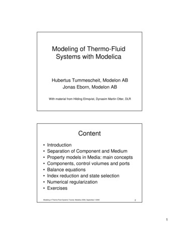
Root function remedy0.10 .10.050 .0 50.960.981.021.040 .9 60 .9 81 .0 21 .0 4-0.05-0.05-0.1-0.1 Replace singular part with local, non-singularsubstitute– result should be qualitatively correct– the overall function should be C1 continuous– No singular derivatives should remain!Modeling of Thermo-Fluid Systems Tutorial, Modelica 2006, September 4 200637Log-mean TemperatureLog-mean Temperature Tlm T1 T2ln( T1 / T2 ) Invalid for all sign( T1 ) sign( T2 ) 0 numerical singularities for T1 T2 , T1 0, T2 0Modeling of Thermo-Fluid Systems Tutorial, Modelica 2006, September 4 20063819
Log-mean Temperature DifferenceBoundaries withridgesRed areas:log-mean invalid T1 T2singularityDynamic models can bein any quadrant!Boundaries withinfinite derivativeModeling of Thermo-Fluid Systems Tutorial, Modelica 2006, September 4 200639Scaling Scale extremely nonlinear functions toimprove numerical behavior. Use min, max and nominal attributes sothat the solver can scale.Real myVar(min 1.0e-10, max 1.0, nominal 1e-3)Modeling of Thermo-Fluid Systems Tutorial, Modelica 2006, September 4 20064020
Scaling: chemical equilibrium ofdissociation of Hydrogen1H 2 H2xH xH2pexp( k )k 2.6727 11.247 0.0743 T 0.4317log(T ) 0.002407 T 2TTake the log of the equation and variables:log( xH ) 1(log( xH2 ) log( p )) k2Modeling of Thermo-Fluid Systems Tutorial, Modelica 2006, September 4 200641Scaling: chemical equilibrium ofdissociation of Hydrogen1H 2 H2Effect of log at 280K: ratio ofratio ofxH2xH 1.3 1075log( xH 2 )log( xH ) 172Experiences tested with several non-linear solvers:22 simultaneous, similar equilibrium reactionsexp form: solvable if T 1200 Klog form: solvable if T 250 KModeling of Thermo-Fluid Systems Tutorial, Modelica 2006, September 4 20064221
Smoothing Piece-wise and discontinuous functionapproximations which should be continuousfor physical reasons shall be smoothened.Modeling of Thermo-Fluid Systems Tutorial, Modelica 2006, September 4 200643Smoothing example:Heat transfer equations Convective heat transfer with flow perpendicularto a cylinder. Two Nusselt numbers for laminarand turbulent flowNulam 0.664 Re1/ 2 Pr1 / 3Nuturb 0.80.037 Re Pr1 2.443Re 0.1 ( Pr 2 / 3 1)For Re 10 wehave to take careof the root functionsingularity as well! Combine as:22Nu 0.3 Nulam Nuturb10 Re 107 , 0.6 Pr 1000Modeling of Thermo-Fluid Systems Tutorial, Modelica 2006, September 4 20064422
SummaryFramework for object-oriented fluid modeling Media and component models decoupled Reversing flows Ideal models for mixing and separation Index reduction for– transformations of media equations– handling of incompressible media– Index reduction for combining volumes Some issues in numerical regularizationModeling of Thermo-Fluid Systems Tutorial, Modelica 2006, September 4 200645Exercises1.Build up small model and run with different media–––2.Look at state selectionCheck non-linear equation systemsTest different options for incompressible mediaReversing flow and singularity treatment––3.Build up model with potential backflowTest with regularized and Text-book version of pressure dropIndex reduction and efficient state selection with fluid models, 3different examples1.2.3.4.5.Index reduction through temperature constraint of solid body and fluidvolume (used in power plant modeling)Index reduction between 2 well mixed volumesIndex reduction between tanks without a pressure drop in between.Non-linear equation systems in networks of simple pressure lossesReversing and 0-flow with liquid valve modelsModeling of Thermo-Fluid Systems Tutorial, Modelica 2006, September 4 20064623
Exercises All exercises are explained step by step in the infolayer in Dymola of the corresponding exercise models.All models are prepared and can be run directly, thethe exercises modify and explore the modelsModeling of Thermo-Fluid Systems Tutorial, Modelica 2006, September 4 200647Exercise 1 Using different Media with the same plant and test of0-flow conditionsModeling of Thermo-Fluid Systems Tutorial, Modelica 2006, September 4 20064824
Exercise 2 Effect of Square root singularityModeling of Thermo-Fluid Systems Tutorial, Modelica 2006, September 4 200649Exercise 3-1 Index reduction between solid body and fluid volume1niotcevnoCConstant1k 1Insert and removeconvection modelModeling of Thermo-Fluid Systems Tutorial, Modelica 2006, September 4 20065025
Exercise 3-2 Index reduction between 2 well mixed fluid volumesInsert and removepipe modelModeling of Thermo-Fluid Systems Tutorial, Modelica 2006, September 4 200651Exercise 3-3 Index reduction of one state only between 2 tankmodelsSpecialTa.101325level st.3flow sourceMassFlow So.SpecialTa.101325level st.2pipeRemovepipeSinkmm .duration 2remove pipe modelModeling of Thermo-Fluid Systems Tutorial, Modelica 2006, September 4 20065226
Exercise 4 Non-linear equations in pipe network modelsModeling of Thermo-Fluid Systems Tutorial, Modelica 2006, September 4 200653Exercise 5 Reversing flow for a liquid valveModeling of Thermo-Fluid Systems Tutorial, Modelica 2006, September 4 20065427
Modeling of Thermo-Fluid Systems Tutorial, Modelica 2006, September 4 2006 13 Connectors and Reversible flow Compressible and non-compressible fluids Reversing flows Ideal mixing R.port Component R Component S Component T S.portA S.portB Fluid properties Modeling of Thermo-Fluid Systems Tutorial, Modelica 2006, September 4 2006 14 R .