Transcription
Learning with Noisy LabelsNagarajan NatarajanInderjit S. DhillonPradeep RavikumarDepartment of Computer Science, University of Texas, uj TewariDepartment of Statistics, University of Michigan, Ann Arbor.tewaria@umich.eduAbstractIn this paper, we theoretically study the problem of binary classification in thepresence of random classification noise — the learner, instead of seeing the true labels, sees labels that have independently been flipped with some small probability.Moreover, random label noise is class-conditional — the flip probability dependson the class. We provide two approaches to suitably modify any given surrogateloss function. First, we provide a simple unbiased estimator of any loss, and obtain performance bounds for empirical risk minimization in the presence of iiddata with noisy labels. If the loss function satisfies a simple symmetry condition,we show that the method leads to an efficient algorithm for empirical minimization. Second, by leveraging a reduction of risk minimization under noisy labelsto classification with weighted 0-1 loss, we suggest the use of a simple weightedsurrogate loss, for which we are able to obtain strong empirical risk bounds. Thisapproach has a very remarkable consequence — methods used in practice suchas biased SVM and weighted logistic regression are provably noise-tolerant. Ona synthetic non-separable dataset, our methods achieve over 88% accuracy evenwhen 40% of the labels are corrupted, and are competitive with respect to recentlyproposed methods for dealing with label noise in several benchmark datasets.1 IntroductionDesigning supervised learning algorithms that can learn from data sets with noisy labels is a problemof great practical importance. Here, by noisy labels, we refer to the setting where an adversary hasdeliberately corrupted the labels [Biggio et al., 2011], which otherwise arise from some “clean”distribution; learning from only positive and unlabeled data [Elkan and Noto, 2008] can also be castin this setting. Given the importance of learning from such noisy labels, a great deal of practicalwork has been done on the problem (see, for instance, the survey article by Nettleton et al. [2010]).The theoretical machine learning community has also investigated the problem of learning fromnoisy labels. Soon after the introduction of the noise-free PAC model, Angluin and Laird [1988]proposed the random classification noise (RCN) model where each label is flipped independentlywith some probability ρ [0, 1/2). It is known [Aslam and Decatur, 1996, Cesa-Bianchi et al.,1999] that finiteness of the VC dimension characterizes learnability in the RCN model. Similarly, inthe online mistake bound model, the parameter that characterizes learnability without noise — theLittestone dimension — continues to characterize learnability even in the presence of random labelnoise [Ben-David et al., 2009]. These results are for the so-called “0-1” loss. Learning with convexlosses has been addressed only under limiting assumptions like separability or uniform noise rates[Manwani and Sastry, 2013].In this paper, we consider risk minimization in the presence of class-conditional random label noise(abbreviated CCN). The data consists of iid samples from an underlying “clean” distribution D.The learning algorithm sees samples drawn from a noisy version Dρ of D — where the noise ratesdepend on the class label. To the best of our knowledge, general results in this setting have not beenobtained before. To this end, we develop two methods for suitably modifying any given surrogateloss function ℓ, and show that minimizing the sample average of the modified proxy loss function1
ℓ̃ leads to provable risk bounds where the risk is calculated using the original loss ℓ on the cleandistribution.In our first approach, the modified or proxy loss is an unbiased estimate of the loss function. Theidea of using unbiased estimators is well-known in stochastic optimization [Nemirovski et al., 2009],and regret bounds can be obtained for learning with noisy labels in an online learning setting (SeeAppendix B). Nonetheless, we bring out some important aspects of using unbiased estimators ofloss functions for empirical risk minimization under CCN. In particular, we give a simple symmetrycondition on the loss (enjoyed, for instance, by the Huber, logistic, and squared losses) to ensure thatthe proxy loss is also convex. Hinge loss does not satisfy the symmetry condition, and thus leadsto a non-convex problem. We nonetheless provide a convex surrogate, leveraging the fact that thenon-convex hinge problem is “close” to a convex problem (Theorem 6).Our second approach is based on the fundamental observation that the minimizer of the risk (i.e.probability of misclassification) under the noisy distribution differs from that of the clean distribution only in where it thresholds η(x) P (Y 1 x) to decide the label. In order to correct for thethreshold, we then propose a simple weighted loss function, where the weights are label-dependent,as the proxy loss function. Our analysis builds on the notion of consistency of weighted loss functions studied by Scott [2012]. This approach leads to a very remarkable result that appropriatelyweighted losses like biased SVMs studied by Liu et al. [2003] are robust to CCN.The main results and the contributions of the paper are summarized below:1. To the best of our knowledge, we are the first to provide guarantees for risk minimization underrandom label noise in the general setting of convex surrogates, without any assumptions on thetrue distribution.2. We provide two different approaches to suitably modifying any given surrogate loss function,that surprisingly lead to very similar risk bounds (Theorems 3 and 11). These general resultsinclude some existing results for random classification noise as special cases.3. We resolve an elusive theoretical gap in the understanding of practical methods like biased SVMand weighted logistic regression — they are provably noise-tolerant (Theorem 11).4. Our proxy losses are easy to compute — both the methods yield efficient algorithms.5. Experiments on benchmark datasets show that the methods are robust even at high noise rates.The outline of the paper is as follows. We introduce the problem setting and terminology in Section2. In Section 3, we give our first main result concerning the method of unbiased estimators. InSection 4, we give our second and third main results for certain weighted loss functions. We presentexperimental results on synthetic and benchmark data sets in Section 5.1.1 Related WorkStarting from the work of Bylander [1994], many noise tolerant versions of the perceptron algorithmhave been developed. This includes the passive-aggressive family of algorithms [Crammer et al.,2006], confidence weighted learning [Dredze et al., 2008], AROW [Crammer et al., 2009] and theNHERD algorithm [Crammer and Lee, 2010]. The survey article by Khardon and Wachman [2007]provides an overview of some of this literature. A Bayesian approach to the problem of noisy labelsis taken by Graepel and Herbrich [2000] and Lawrence and Schölkopf [2001]. As Adaboost is verysensitive to label noise, random label noise has also been considered in the context of boosting. Longand Servedio [2010] prove that any method based on a convex potential is inherently ill-suited torandom label noise. Freund [2009] proposes a boosting algorithm based on a non-convex potentialthat is empirically seen to be robust against random label noise.Stempfel and Ralaivola [2009] proposed the minimization of an unbiased proxy for the case ofthe hinge loss. However the hinge loss leads to a non-convex problem. Therefore, they proposedheuristic minimization approaches for which no theoretical guarantees were provided (We addressthe issue in Section 3.1). Cesa-Bianchi et al. [2011] focus on the online learning algorithms wherethey only need unbiased estimates of the gradient of the loss to provide guarantees for learning withnoisy data. However, they consider a much harder noise model where instances as well as labelsare noisy. Because of the harder noise model, they necessarily require multiple noisy copies perclean example and the unbiased estimation schemes also become fairly complicated. In particular,their techniques break down for non-smooth losses such as the hinge loss. In contrast, we showthat unbiased estimation is always possible in the more benign random classification noise setting.Manwani and Sastry [2013] consider whether empirical risk minimization of the loss itself on the2
noisy data is a good idea when the goal is to obtain small risk under the clean distribution. Butit holds promise only for 0-1 and squared losses. Therefore, if empirical risk minimization overnoisy samples has to work, we necessarily have to change the loss used to calculate the empiricalrisk. More recently, Scott et al. [2013] study the problem of classification under class-conditionalnoise model. However, they approach the problem from a different set of assumptions — the noiserates are not known, and the true distribution satisfies a certain “mutual irreducibility” property.Furthermore, they do not give any efficient algorithm for the problem.2 Problem Setup and BackgroundLet D be the underlying true distribution generating (X, Y ) X { 1} pairs from which n iidsamples (X1 , Y1 ), . . . , (Xn , Yn ) are drawn. After injecting random classification noise (independently for each i) into these samples, corrupted samples (X1 , Ỹ1 ), . . . , (Xn , Ỹn ) are obtained. Theclass-conditional random noise model (CCN, for short) is given by:P (Ỹ 1 Y 1) ρ 1 , P (Ỹ 1 Y 1) ρ 1 , and ρ 1 ρ 1 1The corrupted samples are what the learning algorithm sees. We will assume that the noise ratesρ 1 and ρ 1 are known1 to the learner. Let the distribution of (X, Ỹ ) be Dρ . Instances are denotedby x X Rd . Noisy labels are denoted by ỹ.Let f : X R be somefunction. The risk of f w.r.t. the 0-1 loss is given by real-valued decision RD (f ) E(X,Y ) D 1{sign(f (X))6 Y } . The optimal decision function (called Bayes optimal) thatminimizes RD over all real-valued decision functions is given by f (x) sign(η(x) 1/2) whereη(x) P (Y 1 x). We denote by R the corresponding Bayes risk under the clean distributionD, i.e. R RD (f ). Let ℓ(t, y) denote a loss function where t R is a real-valued prediction andy { 1} is a label. Let ℓ̃(t, ỹ) denote a suitably modified ℓ for use with noisy labels (obtained usingmethods in Sections 3 and 4). It is helpful to summarize the three important quantities associatedwith a decision function f :b (f ) : 1 Pn ℓ̃(f (Xi ), Ỹi ).1. Empirical ℓ̃-risk on the observed sample: Ri 1ℓ̃nb (f ) to be close to the ℓ̃-risk under the noisy distribution Dρ :2. As n grows, we expect Rℓ̃hiRℓ̃,Dρ (f ) : E(X,Ỹ ) Dρ ℓ̃(f (X), Ỹ ) .3. ℓ-risk under the “clean” distribution D: Rℓ,D (f ) : E(X,Y ) D [ℓ(f (X), Y )].Typically, ℓ is a convex function that is calibrated with respect to an underlying loss function such asthe 0-1 loss. ℓ is said to be classification-calibrated [Bartlett et al., 2006] if and only if there exists aconvex, invertible, nondecreasing transformation ψℓ (with ψℓ (0) 0) such that ψℓ (RD (f ) R ) Rℓ,D (f ) minf Rℓ,D (f ). The interpretation is that we can control the excess 0-1 risk by controllingthe excess ℓ-risk.If f is not quantified in a minimization, then it is implicit that the minimization is over all measurablefunctions. Though most of our results apply to a general function class F , we instantiate F to be theset of hyperplanes of bounded L2 norm, W {w Rd : kwk2 W2 } for certain specific results.Proofs are provided in the Appendix A.3 Method of Unbiased EstimatorsLet F : X R be a fixed class of real-valued decision functions, over which the empirical risk isminimized. The method of unbiased estimators uses the noise rates to construct an unbiased estimator ℓ̃(t, ỹ) for the loss ℓ(t, y). However, in the experiments we will tune the noise rate parametersthrough cross-validation. The following key lemma tells us how to construct unbiased estimators ofthe loss from noisy labels.Lemma 1. Let ℓ(t, y) be any bounded loss function. Then, if we define,ℓ̃(t, y) : we have, for any t, y,1(1 ρ y ) ℓ(t, y) ρy ℓ(t, y)1 ρ 1 ρ 1hiEỹ ℓ̃(t, ỹ) ℓ(t, y) .This is not necessary in practice. See Section 5.3
We can try to learn a good predictor in the presence of label noise by minimizing the sample averageb (f ) .fˆ argmin Rf Fℓ̃By unbiasedness of ℓ̃ (Lemma 1), we know that, for any fixed f F , the above sample averageconverges to Rℓ,D (f ) even though the former is computed using noisy labels whereas the latterdepends on the true labels. The following result gives a performance guarantee for this procedure interms of the Rademacher complexity of the function class F . The main idea in the proof is to usethe contraction principle for Rademacher complexity to get rid of the dependence on the proxy lossℓ̃. The price to pay for this is Lρ , the Lipschitz constant of ℓ̃.Lemma 2. Let ℓ(t, y) be L-Lipschitz in t (for every y). Then, with probability at least 1 δ,rlog(1/δ)bmax Rℓ̃ (f ) Rℓ̃,Dρ (f ) 2Lρ R(F ) f F2n where R(F ) : EXi ,ǫi supf F n1 ǫi f (Xi ) is the Rademacher complexity of the function class Fand Lρ 2L/(1 ρ 1 ρ 1 ) is the Lipschitz constant of ℓ̃. Note that ǫi ’s are iid Rademacher(symmetric Bernoulli) random variables.The above lemma immediately leads to a performance bound for fˆ with respect to the clean distribution D. Our first main result is stated in the theorem below.Theorem 3 (Main Result 1). With probability at least 1 δ,rlog(1/δ)ˆ.Rℓ,D (f ) min Rℓ,D (f ) 4Lρ R(F ) 2f F2nFurthermore, if ℓ is classification-calibrated, there exists a nondecreasing function ζℓ with ζℓ (0) 0such that,r log(1/δ) ˆRD (f ) R ζℓ min Rℓ,D (f ) min Rℓ,D (f ) 4Lρ R(F ) 2.f Ff2nThe term on the right hand side involves both approximation error (that is small if F is large) andestimation error (that is small if F is small). However, by appropriately increasing the richness ofthe class F with sample size, we can ensure that the misclassification probability of fˆ approachesthe Bayes risk of the true distribution. This is despite the fact that the method of unbiased estimatorscomputes the empirical minimizer fˆ on a sample from the noisy distribution. Getting the optimalempirical minimizer fˆ is efficient if ℓ̃ is convex. Next, we address the issue of convexity of ℓ̃.3.1 Convex losses and their estimatorsNote that the loss ℓ̃ may not be convex even if we start with a convex ℓ. An example is providedby the familiar hinge loss ℓhin (t, y) [1 yt] . Stempfel and Ralaivola [2009] showed that ℓ̃hin isnot convex in general (of course, when ρ 1 ρ 1 0, it is convex). Below we provide a simplecondition to ensure convexity of ℓ̃.Lemma 4. Suppose ℓ(t, y) is convex and twice differentiable almost everywhere in t (for every y)and also satisfies the symmetry property t R, ℓ′′ (t, y) ℓ′′ (t, y) .Then ℓ̃(t, y) is also convex in t.Examples satisfying the conditions of the lemma above are the squared loss ℓsq (t, y) (t y)2 , thelogistic loss ℓlog (t, y) log(1 exp( ty)) and the Huber loss: if yt 1 4ytℓHub (t, y) (t y)2 if 1 yt 1 0if yt 1Consider the case where ℓ̃ turns out to be non-convex when ℓ is convex, as in ℓ̃hin . In the onlinelearning setting (where the adversary chooses a sequence of examples, and the prediction of a learnerat round i is based on the history of i 1 examples with independently flipped labels), we coulduse a stochastic mirror descent type algorithm [Nemirovski et al., 2009] to arrive at risk bounds (SeeAppendix B) similar to Theorem 3. Then, we only need the expected loss to be convex and therefore4
ℓhin does not present a problem. At first blush, it may appear that we do not have much hope ofobtaining fˆ in the iid setting efficiently. However, Lemma 2 provides a clue.b (w) is non-convex, itWe will now focus on the function class W of hyperplanes. Even though Rℓ̃b (w) is uniformlyis uniformly close to Rℓ̃,Dρ (w). Since Rℓ̃,Dρ (w) Rℓ,D (w), this shows that Rℓ̃close to a convex function over w W. The following result shows that we can therefore approxb (w) by minimizing the biconjugate F . Recall that the (Fenchel)imately minimize F (w) Rℓ̃ biconjugate F is the largest convex function that minorizes F .Lemma 5. Let F : W R be a non-convex function defined on function class W such it is ε-closeto a convex function G : W R: w W, F (w) G(w) εThen any minimizer of F is a 2ε-approximate (global) minimizer of F .Now, the following theorem establishes bounds for the case when ℓ̃ is non-convex, via the solutionobtained by minimizing the convex function F .Theorem 6. Let ℓ be a loss, such as the hinge loss, for which ℓ̃ is non-convex. Let W {w :kw2 k W2 }, let kXi k2 X2 almost surely, and let ŵapprox be any (exact) minimizer of theconvex problemmin F (w) ,w Wb (w). Then, with probabilitywhere F (w) is the (Fenchel) biconjugate of the function F (w) Rℓ̃bat least 1 δ, ŵapprox is a 2ε-minimizer of Rℓ̃ (·) wherer2Lρ X2 W2log(1/δ) ε .n2nTherefore, with probability at least 1 δ,Rℓ,D (ŵapprox ) min Rℓ,D (w) 4ε .w WNumerical or symbolic computation of the biconjugate of a multidimensional function is difficult,in general, but can be done in special cases. It will be interesting to see if techniques from Computational Convex Analysis [Lucet, 2010] can be used to efficiently compute the biconjugate above.4 Method of label-dependent costsWe develop the method of label-dependent costs from two key observations. First, the Bayes classifier for noisy distribution, denoted f , for the case ρ 1 6 ρ 1 , simply uses a threshold differentfrom 1/2. Second, f is the minimizer of a “label-dependent 0-1 loss” on the noisy distribution. Theframework we develop here generalizes known results for the uniform noise rate setting ρ 1 ρ 1and offers a more fundamental insight into the problem. The first observation is formalized in thelemma below.Lemma 7. Denote P (Y 1 X) by η(X) and P (Ỹ 1 X) by η̃(X).The Bayes classifier under the noisy distribution, f argminf E(X,Ỹ ) Dρ 1{sign(f (X))6 Ỹ } is given by, 1/2 ρ 1.f (x) sign(η̃(x) 1/2) sign η(x) 1 ρ 1 ρ 1Interestingly, this “noisy” Bayes classifier can also be obtained as the minimizer of a weighted 0-1loss; which as we will show, allows us to “correct” for the threshold under the noisy distribution.Let us first introduce the notion of “label-dependent” costs for binary classification. We can writethe 0-1 loss as a label-dependent loss as follows:1{sign(f (X))6 Y } 1{Y 1} 1{f (X) 0} 1{Y 1} 1{f (X) 0}We realize that the classical 0-1 loss is unweighted. Now, we could consider an α-weighted versionof the 0-1 loss as:Uα (t, y) (1 α)1{y 1} 1{t 0} α1{y 1} 1{t 0} ,where α (0, 1). In fact we see that minimization w.r.t. the 0-1 loss is equivalent to that w.r.t.U1/2 (f (X), Y ). It is not a coincidence that Bayes optimal f has a threshold 1/2. The followinglemma [Scott, 2012] shows that in fact for any α-weighted 0-1 loss, the minimizer thresholds η(x)at α.5
Lemma 8 (α-weighted Bayes optimal [Scott, 2012]). Define Uα -risk under distribution D asRα,D (f ) E(X,Y ) D [Uα (f (X), Y )].Then, fα (x) sign(η(x) α) minimizes Uα -risk.Now consider the risk of f w.r.t. the α-weighted 0-1 loss under noisy distribution Dρ : Rα,Dρ (f ) E(X,Ỹ ) Dρ Uα (f (X), Ỹ ) .At this juncture, we are interested in the following question: Does there exist an α (0, 1) suchthat the minimizer of Uα -risk under noisy distribution Dρ has the same sign as that of the Bayesoptimal f ? We now present our second main result in the following theorem that makes a strongerstatement — the Uα -risk under noisy distribution Dρ is linearly related to the 0-1 risk under theclean distribution D. The corollary of the theorem answers the question in the affirmative.Theorem 9 (Main Result 2). For the choices,1 ρ 1 ρ 11 ρ 1 ρ 1α and Aρ ,22there exists a constant BX that is independent of f such that, for all functions f ,Rα ,Dρ (f ) Aρ RD (f ) BX . Corollary 10. The α -weighted Bayes optimal classifier under noisy distribution coincides withthat of 0-1 loss under clean distribution:argmin Rα ,Dρ (f ) argmin RD (f ) sign(η(x) 1/2).ff4.1 Proposed Proxy Surrogate LossesConsider any surrogate loss function ℓ; and the following decomposition:ℓ(t, y) 1{y 1} ℓ1 (t) 1{y 1} ℓ 1 (t)where ℓ1 and ℓ 1 are partial losses of ℓ. Analogous to the 0-1 loss case, we can define α-weightedloss function (Eqn. (1)) and the corresponding α-weighted ℓ-risk. Can we hope to minimize an αweighted ℓ-risk with respect to noisy distribution Dρ and yet bound the excess 0-1 risk with respectto the clean distribution D? Indeed, the α specified in Theorem 9 is precisely what we need. We areready to state our third main result, which relies on a generalized notion of classification calibrationfor α-weighted losses [Scott, 2012]:Theorem 11 (Main Result 3). Consider the empirical risk minimization problem with noisy labels:n1Xℓα (f (Xi ), Ỹi ).fˆα argminn i 1f FDefine ℓα as an α-weighted margin loss function of the form:ℓα (t, y) (1 α)1{y 1} ℓ(t) α1{y 1} ℓ( t)(1)where ℓ : R [0, ) is a convex loss function with Lipschitz constant L such that it is classification′calibrated (i.e. ℓ (0) 0). Then, for the choices α and Aρ in Theorem 9, there exists a nondecreasing function ζℓα with ζℓα (0) 0, such that the following bound holds with probability atleast 1 δ:r log(1/δ) 1ˆRD (fα ) R Aρ ζℓα min Rα ,Dρ (f ) min Rα ,Dρ (f ) 4LR(F ) 2.ff F2nAside from bounding excess 0-1 risk under the clean distribution, the importance of the above theorem lies in the fact that it prescribes an efficient algorithm for empirical minimization with noisylabels: ℓα is convex if ℓ is convex. Thus for any surrogate loss function including ℓhin , fˆα can beefficiently computed using the method of label-dependent costs. Note that the choice of α aboveis quite intuitive. For instance, when ρ 1 ρ 1 (this occurs in settings such as Liu et al. [2003]where there are only positive and unlabeled examples), α 1 α and therefore mistakes onpositives are penalized more than those on negatives. This makes intuitive sense since an observednegative may well have been a positive but the other way around is unlikely. In practice we do notneed to know α , i.e. the noise rates ρ 1 and ρ 1 . The optimization problem involves just oneparameter that can be tuned by cross-validation (See Section 5).6
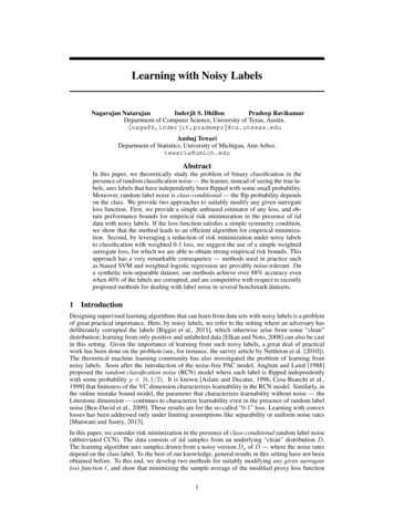
5 ExperimentsWe show the robustness of the proposed algorithms to increasing rates of label noise on synthetic andreal-world datasets. We compare the performance of the two proposed methods with state-of-the-artmethods for dealing with random classification noise. We divide each dataset (randomly) into 3training and test sets. We use a cross-validation set to tune the parameters specific to the algorithms.Accuracy of a classification algorithm is defined as the fraction of examples in the test set classifiedcorrectly with respect to the clean distribution. For given noise rates ρ 1 and ρ 1 , labels of thetraining data are flipped accordingly and average accuracy over 3 train-test splits is computed2. Forevaluation, we choose a representative algorithm based on each of the two proposed methods — ℓ̃logfor the method of unbiased estimators and the widely-used C-SVM [Liu et al., 2003] method (whichapplies different costs on positives and negatives) for the method of label-dependent costs.5.1 Synthetic dataFirst, we use the synthetic 2D linearly separable dataset shown in Figure 1(a). We observe fromexperiments that our methods achieve over 90% accuracy even when ρ 1 ρ 1 0.4. Figure 1shows the performance of ℓ̃log on the dataset for different noise rates. Next, we use a 2D UCIbenchmark non-separable dataset (‘banana’). The dataset and classification results using C-SVM(in fact, for uniform noise rates, α 1/2, so it is just the regular SVM) are shown in Figure 2. Theresults for higher noise rates are impressive as observed from Figures 2(d) and 2(e). The ‘banana’dataset has been used in previous research on classification with noisy labels. In particular, theRandom Projection classifier [Stempfel and Ralaivola, 2007] that learns a kernel perceptron in thepresence of noisy labels achieves about 84% accuracy at ρ 1 ρ 1 0.3 as observed fromour experiments (as well as shown by Stempfel and Ralaivola [2007]), and the random hyperplanesampling method [Stempfel et al., 2007] gets about the same accuracy at (ρ 1 , ρ 1 ) (0.2, 0.4) (asreported by Stempfel et al. [2007]). Contrast these with C-SVM that achieves about 90% accuracyat ρ 1 ρ 1 0.2 and over 88% accuracy at ρ 1 ρ 1 020202000000 20 20 20 20 20 40 40 40 40 40 60 60 60 80 80 100 100 80 60 40 20020406080100 100 100 60 80 80 60 40(a) 20020406080100 100 10020 60 80 80 60 40(b) 20020406080100 100 100 80 80 60 40(c) 20020406080100 100 100 80 60 40(d) 20020406080100(e)Figure 1: Classification of linearly separable synthetic data set using ℓ̃log . The noise-free data isshown in the leftmost panel. Plots (b) and (c) show training data corrupted with noise rates (ρ 1 ρ 1 ρ) 0.2 and 0.4 respectively. Plots (d) and (e) show the corresponding classification results.The algorithm achieves 98.5% accuracy even at 0.4 noise rate per class. (Best viewed in color).4444433333222221111100000 1 1 1 1 1 2 2 2 2 2 3 4 3 2 1(a)0123 3 4 3 2 1(b)0123 3 4 3 2 10(c)123 3 4 3 2 1(d)0123 3 4 3 2 10123(e)Figure 2: Classification of ‘banana’ data set using C-SVM. The noise-free data is shown in (a). Plots(b) and (c) show training data corrupted with noise rates (ρ 1 ρ 1 ρ) 0.2 and 0.4 respectively.Note that for ρ 1 ρ 1 , α 1/2 (i.e. C-SVM reduces to regular SVM). Plots (d) and (e) showthe corresponding classification results (Accuracies are 90.6% and 88.5% respectively). Even when40% of the labels are corrupted (ρ 1 ρ 1 0.4), the algorithm recovers the class structures asobserved from plot (e). Note that the accuracy of the method at ρ 0 is 90.8%.5.2 Comparison with state-of-the-art methods on UCI benchmarkWe compare our methods with three state-of-the-art methods for dealing with random classification noise: Random Projection (RP) classifier [Stempfel and Ralaivola, 2007]), NHERD2Note that training and cross-validation are done on the noisy training data in our setting. To account forrandomness in the flips to simulate a given noise rate, we repeat each experiment 3 times — independentcorruptions of the data set for same setting of ρ 1 and ρ 1 , and present the mean accuracy over the trials.7
DATASET (d, n , n )Breast cancer(9, 77, 186)Diabetes(8, 268, 500)Thyroid(5, 65, 150)German(20, 300, 700)Heart(13, 120, 150)Image(18, 1188, 898)Noise ratesρ 1 ρ 1 0.2ρ 1 0.3, ρ 1 0.1ρ 1 ρ 1 0.4ρ 1 ρ 1 0.2ρ 1 0.3, ρ 1 0.1ρ 1 ρ 1 0.4ρ 1 ρ 1 0.2ρ 1 0.3, ρ 1 0.1ρ 1 ρ 1 0.4ρ 1 ρ 1 0.2ρ 1 0.3, ρ 1 0.1ρ 1 ρ 1 0.4ρ 1 ρ 1 0.2ρ 1 0.3, ρ 1 0.1ρ 1 ρ 1 0.4ρ 1 ρ 1 0.2ρ 1 0.3, ρ 1 0.1ρ 1 ρ 1 479.2668.1565.2970.6664.72Table 1: Comparative study of classification algorithms on UCI benchmark datasets. Entries within1% from the best in each row are in bold. All the methods except NHERD variants (whichare not kernelizable) use Gaussian kernel with width 1. All method-specific parameters are estimated through cross-validation. Proposed methods (ℓ̃log and C-SVM) are competitive across all thedatasets. We show the best performing NHERD variant (‘project’ and ‘exact’) in each case.[Crammer and Lee, 2010]) (project and exact variants3 ), and perceptron algorithm with margin (PAM) which was shown to be robust to label noise by Khardon and Wachman [2007].We use the standard UCI classification datasets, preprocessed and made available by ). For kernelized algorithms, we useGaussian kernel with width set to the best width obtained by tuning it for a traditional SVM onthe noise-free data. For ℓ̃log , we use ρ 1 and ρ 1 that give the best accuracy in cross-validation. ForC-SVM, we fix one of the weights to 1, and tune the other. Table 1 shows the performance of themethods for different settings of noise rates. C-SVM is competitive in 4 out of 6 datasets (Breastcancer, Thyroid, German and Image), while relatively poorer in the other two. On the other hand,ℓ̃log is competitive in all the data sets, and performs the best more often. When about 20% labels arecorrupted, uniform (ρ 1 ρ 1 0.2) and non-uniform cases (ρ 1 0.3, ρ 1 0.1) have similaraccuracies in all the data sets, for both C-SVM and ℓ̃log . Overall, we observe that the proposedmethods are competitive and are able to tolerate moderate to high amounts of label noise in the data.Finally, in domains where noise rates are approximately known, our methods can benefit from theknowledge of noise rates. Our analysis shows that the methods are fairly robust to misspecificationof noise rates (See Appendix C for results).6 Conclusions and Future WorkWe addressed the problem of risk minimization in the presence of random classification noise, andob
NHERD algorithm [Crammer and Lee, 2010]. The survey article by Khardon and Wachman [2007] provides an overview of some of this literature. A Bayesian approach to the problem of noisy labels is taken by Graepel and Herbrich [2000] and Lawrence and Sch olkopf [2001]. As Adaboost is very