WIXLIB

Spin, which is the most basic two-valued quantum attribute, is missing from aspatial description. This subtle degree of freedom, whose existence is deducedby analysis of the Stern-Gerlach experiment, is an additional Hilbert spacevector feature. For example, for a single spin 1/2 system the wave functionincluding both space and spin aspects is:Ψ( r1 , t) s ms ,(1)where s ms denotes a state that is simultaneously an eigenstate of theparticle’s total spin operator s2 s2x s2y s2z , and of its spin componentoperator sz . That iss2 sms h̄2 s(s 1) sms sz sms h̄ms sms .(2)For a spin 1/2 system, we denote the spin up state as sms 12 , 12 0 ,and the spin down state as sms 21 , 21 1 .We now arrive at the definition of a one qubit state as a superposition of thetwo states associated with the above 0 and 1 bits: Ψ a 0 b 1 ,(3)where a 0 Ψ and b 1 Ψ are complex probability amplitudes forfinding the particle with spin up or spin down, respectively. The normalizationof the state Ψ Ψ 1, yields a 2 b 2 1. Note that the spatialaspects of the wave function are being suppressed; which corresponds to theparticles being in a fixed location, such as at quantum dots. 2An essential point is that a QM system can exist in a superposition of thesetwo bits; hence, the state is called a quantum-bit or “qubit.” Although ourdiscussion uses the notation of a system with spin, it should be noted that thesame discussion applies to any two distinct states that can be associated with 0 and 1 . Indeed, the following section on the Pauli spin operators isreally a description of any system that has two recognizable states.2.0.1 UsageQDENSITY includescommands for qubit states as ket and bra vectors. For example, commands Ket[0], Bra[0],Ket[1], Bra[1], yield2When these separated systems interact, one might need to restore the spatialaspects of the full wave function.7

In[1] : Ket[0] 1 Out[1] : 0In[2] : Ket[1] 0 Out[2] : 1In[3] : Bra[0]Out[3] : (1 0)In[4] : Bra[1]Out[4] : (0 1)These are the computational basis states, i.e. eigenstates of the spin operatorin the z-direction.States that are eigenstates of the spin operator in the x-direction are invokedby the commandsIn[5] : BraX[0] 11Out[5] : 22which is equivalent to: In[6] : (Bra[0] Bra[1])/ 2 11Out[6] : 22Eigenstates of the spin operator in the y-direction are invoked similarly thecommands BraY[0], BraY[1], etc.8

2.1 The Pauli Spin OperatorWe use the case of a spin 1/2 particle to describe a quantum system withtwo discrete levels; the same description can be applied to any QM systemwith two distinct levels. The spin s operator is related to the three Pauli spinoperators σx , σy , σz byh̄(4) s ( ) σ ,2from which we see that σ is an operator that describes the spin 1/2 systemin units of h̄2 . Since spin is an observable, it is represented by a Hermitianoperator, σ † σ . We also know that measurement of spin is subject to theuncertainty principle, which is reflected in the non-commuting operator properties of spin and hence of the Pauli operators. For example, from the standardcommutator property for any spin [sx , sy ] ih̄sz , one deduces that the Paulioperators do not commute[σx , σy ] 2iσz .This holds for all cyclic components so we have a general form[σi , σj ] 2i ijk σk .(5)3(6)An important property of the spin algebra is that the total spin commutes withany component of the spin operator [s2 , si ] 0 for all i. The physical consequence is that one can simultaneously measure the total spin of the systemand one component (usually sz ) of the spin. Only one component is a candidate for simultaneous measurement because the commutator [sx , sy ] ih̄szis already an uncertainty principle constraint on the other components. As aresult of the ability to measure s2 and sz simultaneously, the allowed states ofthe spin 1/2 system are restricted to being spin-up and spin-down with respectto a specified fixed direction ẑ, called the axis of quantization. States definedrelative to that fixed axis are called “computational basis” states, in the QCjargon. The designation arises because as noted already one can identify spinup with a state 0 , which designates the digit or bit 0, and a spin-downstate as 1 , which designates the digit or bit 1.The fact that there are just two states (up and down) also implies propertiesof the Pauli operators. We construct 4 the raising and lowering operators3Here the Levi-Civita symbol is nonzero only for cyclic order of componentsijk xyz, yzx, zxy, for which ijk 1. For anti-cyclic order of componentsijk xzy, zyx, yxz ijk 1. It is otherwise zero.4 With the definition s s is , and using the original spin commutation rules, xyit follows that [s , sz ] s , which reveals that s and hence also σ are raising9

σ σx iσy , and note that the raising and lower process is boundedσ 0 0σ 1 0.(7)Hence, raising a two-valued state up twice or lowering it twice yields a null(unphysical) Hilbert space; this property tells us additional aspects of thePauli operator. Sinceσ σ (σx iσy )2 σx2 σy2 (σx σy σy σx ) 0,(8)we deduce that σx2 σy2 , and that the anti-commutator{σx , σy } σx σy σy σx 0.(9)The anti-commutation property is thus a direct consequence of the restrictionto two levels.The spin 1/2 property is often expressed as: s2 sms h̄2 s(s 1) sms 23 2h̄ sms h̄4 σ 2 sms . We have σ 2 3 σx2 σy2 σz2 2σx2 1, where4we use the above equality σx2 σy2 , and from the ẑ eigenvalue equation theproperty σz2 1, to deduce thatσx2 σy2 σz2 1.(10)Another useful property of the Pauli matrices is obtained by combining theabove properties and commutator and anti-commutator into one expressionfor a given spin 1/2 systemσi σj δij i ijk σk ,(11)where indices i, j, k take on the values x, y, z, and repeated indices are assumedto be summed over. For two general vectors, this becomes σ · B) A ·B i(A B) · σ .( σ · A)( (12) B η, a unit vector ( σ · η)2 1, which will be useful later.For AThese operator properties can also be represented by the Pauli-spin matrices,where we identify the matrix elements by 1 0 s m0s σz s ms 0 1 .(13)and lowering operators.The general result, including the limit on the total spin isps s ms s(s 1) ms (ms 1) s ms 1 .10

Similarly for the x and y component spin operators 0 sm0s σx s ms 1 1 0 0 sm0s σy sms These are all Hermitian matrices σi i i 0σi† . .(14)Also, the matrix realization for the raising and lowering operators are: 0 0 σ .2 00 2 σ 0 0(15)†Here σ σ .Note that these 2 2 Pauli matrices are traceless Tr[ σ ] 0, unimodular σi2 1and have unit determinant det σi 1. Along with the unit operator 1σ0 1 0 0 1 ,(16)the four Pauli operators form a basis for the expansion of any spin operator inthe single qubit space. For example, we can express the rotation of a spin assuch an expansion and later we shall introduce a density matrix for a singlequbit in the form ρ a b · σ a b n · σ to describe an ensemble of particlespin directions as occurs in a beam of spin-1/2 particles.In QDENSITY , we denote the four matrices by σi where i 0 is the unit matrixand i 1, 2, 3 corresponds to the components x, y, and z. To produce thePauli spin operators in QDENSITY , one can use either the Greek form or theexpression s[i].2.1.1 UsageQDENSITY includescommands for the Pauli operators. For example, there arethree equivalent ways to invoke the Pauli σy matrix in QDENSITY :In[7] : σy 0 i Out[7] : i 0 11

In[8] : s[2] 0 i Out[8] : i 0The third way is to use the commands Sigma0, Sigma1,Sigma2, or Sigma3.Note thatIn[9] : σ2 . KetY[0] KetY[0] 0 Out[9] : 0andIn[10] : σ2 . KetY[1] KetY[1] 0 Out[10] : 0confirm that KetY[0] and KetY[1] are indeed eigenstates of σy . Note thatthe · is used to take the dot product.2.2 Pauli Operators in Hilbert SpaceIt is often convenient to express the above matrix properties in the form ofoperators in Hilbert space. For a general operator Ω, using closure, we haveΩ XXnn0 n n Ω n0 n0 .(17)For the four Pauli operators this yields:σ0 0 0 1 1 σ1 0 1 1 0 σ2 i 0 1 i 1 0 σz 0 0 1 1 .(18)12

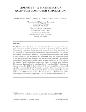
Taking matrix elements of these operators reproduces the above Pauli matrices. Also note we have the general trace propertyTr a b XnX n a b n n b n n a b a ,(19)where n is a complete orthonormal (CON) basis . Applying this trace ruleto the above operator expressions confirms that Tr[σx ] Tr[σy ] Tr[σz ] 0,and Tr[σ0 ] 2.5Another useful trace rule is Tr[ Ω a b ] b Ω a .2.3 Rotation of SpinAnother way to view the above superposition, or qubit, state is that a stateoriginally in the ẑ direction 0 , has been rotated to a new direction specifiedby a unit vector n̂ (nx , ny , nz ) (sin θ cos φ, sin θ sin φ, cos θ), as shown inFig. 1. 0 zθznηθyφy(a)x(b)xFig. 1. Active rotation to a direction n̂ (a); and active rotation around a vector η̂(b).The rotated spin state iφ/2 cos(θ/2)e n̂ cos(θ/2)e iφ/2 0 sin(θ/2)e iφ/2 1 sin(θ/2)e iφ/2 ,(20)is a normalized eigenstate of the operator nz σ · n̂ nx inynx iny nz cos θ sin θe iφ sin θeiφ cos θ .(21)We see that σ · n̂ n̂ n̂ .5For a CON basis, we have closurePn n n 1.13(22)

The half angles above reflect the so-called spinor nature of the QM state ofa spin 1/2 particle in that a double full rotation is needed to bring the wavefunction back to its original form.These rotated spin states allow us to pick a different axis of quantization n̂ foreach particle in an ensemble of spin 1/2 systems. These states are normalized n̂ n̂ 1, but are not orthogonal n̂0 n̂ 6 1, when the n̂ angles θ, φdo not equal the n̂0 angles θ 0 , φ0 .Special cases of the above states with spin pointing in the directions x̂ and ŷ are within phases: 1 1 0 1 x , 2 12 0 i 1 1 1 y .2 i2(23)Hilbert space versions are also shown above.Rotation can also be expressed as a rotation of an initial spin-up system aboutγa rotation axis η̂ by an angle γ. Thus an operator Rγ e i 2 σ ·η̂ , acting as Ψ Rγ 0 (24)can also rotate the spin system state to new direction. This rotation operatorcan be expanded in the formγRγ e i 2 σ·η̂ cosγγσ0 i sin σ · η̂,22(25)which follows from the property that ( σ · η̂)2 η̂ · η̂ i(η̂ η̂) · σ 1 . A specialcase of the state generated by this rotation Rγ 0 is a γ π/2 rotationabout the η̂ ŷ axis. Then the rotation operator isπππRπ/2 e i 4 σy cos σ0 i sin σy .44(26)Introducing the Pauli matrices, this becomesRπ/2 1 1 1 .2 1 114(27)

This rotation about an axis again yields the same result; namely, 1 1 1 1 1 1 1 Rπ/2 0 · .2 1 12 02 1(28)Similar steps apply for a rotation about the x̂ axis by γ π/2, which yieldsthe earlier y states.From normalization of the rotated state Ψ Ψ 0 Rγ† Rγ 0 0 0 1, we see that the rotation is a unitary Rγ† Rγ 1 operator.2.3.1 UsageThe trace of the Pauli operators is invoked inQDENSITY by:In[1] : Tr[σ2 ]Out[1] : 0Rotation about the X axis is represented byIn[2] : RotX[θ] CosOut[2] : h iθ2 iSinh iθ2 iSinCosh i h iθ2θ2 Commands for other directions are described in Tutorial.nb; see RotX[θ],RotY[θ], Rotqbit[vec,θ].2.4 One Qubit ProjectionFor a one qubit system, it is simple to define operators that project on to thespin-up or spin-down states. These projection operators are:P0 0 0 P1 1 1 .15(29)

These are Hermitian operators, and by virtue of closure, sum to oneThey can also be expressed in terms of the σz operator asP0 1 σz2P1 1 σz,2Pa 0,1Pa 1.(30)or in matrix form 1P0 0 0 0 0 0 P1 0 1 .(31)One can also project to other directions. For example, projection of a qubiton to the x̂ or ŷ directions involves the projection operators1 σx,21 σy.P y ŷ ŷ 2P x x̂ x̂ (32)2.4.1 UsageThe above projections operators are invoked inIn[1] : P0 1Out[1] : QDENSITY by: 0 0 0In[2] : P1 0 0 Out[2] : 0 1 Projection operators using the x-basis are invoked by:In[3] : PX[0] Out[3] : 12121212 16

In[4] : PX[1] Out[4] : 12 12 21 12 A general operator ProjG[a,vec] to project into a direction stipulated by aunit three vector vec, with a 0 or 1, is also provided. See Tutorial.nb for moreexamples. These operators are useful for projective measurements.3THE (SPIN) DENSITY MATRIXThe above spin rotated wave functions can be used to obtain the expectationvalue of some relevant Hermitian operator Ω Ω† , which represents a physicalobservable. Let us assume that a system is in a state labelled by α with a statevector α . In general the role of the label α could be to denote a spatialcoordinate (or a momentum), if we were considering an ensemble of localizedparticles. For the spin density matrix, we use α to label the various spindirections n̂.The average or expectation value of a general observable Ω is then α Ω α .This expectation value can be interpreted simply by invoking eigenstates ofthe operator ΩΩ ν ων ν ,(33)where ων are real eigenvalues and ν are the eigenstates, which are usuallya complete orthonormal basis (CON). The physical meaning of the eigenvalueequation is that if the system is in the eigenstate ν , there is no uncertainty Ω in determining the eigenvalue, e.g.( Ω)2 ν Ω2 ν ν Ω ν 2 ων2 ων2 0.(34)Using the eigenstates ν , we can now see the basic meaning of the expectation value, which is a fundamental part of QM. The eigenstates form a CONbasis. That means any function can be expanded in this basis and that thecoefficients can be obtained by an overlap integral. For example, in generalterms the completeness (C) allows the expansion Ψ Xνcν ν .(35)The OrthoNormal (ON) aspect is ν ν 0 δνν 0 . Thus ν 0 Ψ Xνcν ν 0 ν c ν 0 ,17(36)

reinserting this yields Ψ Xν ν Ψ ν Xν ν ν Ψ I Ψ .Thus we see completeness with orthonormality of the basis can be expressedin the closure formX ν ν I,(37)νwith I the unit operator in the Hilbert space.With closure (e.g. a CON basis), we can now see that the expectation valuebreaks in to a sum of the form α Ω α XXνXνν0 α ν ν Ω ν 0 ν 0 α ων ν α α ν Xνων Pαν .Here Pαν ν α α ν ν α 2 is the positive real probability ofthe state α being in the eigenstate ν . Hence we see that the quantumaverage or expectation value is a sum of that probability times the associatedeigenvalue ων over all possible values ν. That is the characteristic of a quantumaverage.As the next step towards the spin density matrix, consider the case that wehave an ensemble of such quantum systems. Each system is considered notto have quantum interference with the other members of the ensemble. Thatsituation can be realized by the ensemble being located at separate sites withnon-overlapping localized wave packets and also in the case of a low densitybeam, i.e. separated particles in the beam. This allows us to take a classicalaverage over the ensemble.Suppose that the first member of the ensemble is produced in the state α ,the next in α0 , etc. The ensemble average is then a simple classical average Ω Pα α Ω α Pα,Pα Pα(38)where Pα is the probability that a particular state α appears in the ensemPble. Summing over all possible states of course yields α Pα 1. The aboveexpression is a combination of a classical ensemble average with the quantummechanical expectation value. It contains the idea that each member of theensemble interferes only with itself quantum mechanically and that the ensemble involves a simple classical average over the probability distribution ofthe ensemble.18

We are close to introducing the density matrix. This is implemented by usingclosure and rearranging. ConsiderXα α Ω α Pα X Xα α m m Ω m0 m0 α Pα ,mm0(39)where m denotes any CON basis. Now rearrange the above toXα α Ω α Pα XX m0 α α m Pα m Ω m0 ,mm0 α(40)and then define the density operator byρ Xα α α Pα(41)and the associated density matrix in the CON basis m as m ρ m0 0α m α α m Pα . We often refer to either the density operatoror the density matrix simply as the “density matrix,” albeit one acts in theHilbert space and the other is an explicit matrix. The ensemble average cannow be expressed as a ratio of traces 6PTr[ρΩ],Tr[ρ] Ω (42)which entails the properties thatTr[ρ] Xm m ρ m αPα α α XXαXPαXm α m m α Pα 1,(43)αandTr[ρΩ] Xmm0 m ρ m0 m0 Ω m XXPα α m0 m0 Ω m m α αmm0αPα α Ω α ,X(44)which returns the original ensemble average expression.6The trace Tr is defined as the sum of the diagonal matrix elements of an operator,where a CON basis is used.19

3.1 Properties of the Density MatrixWe have defined the density operator by a sum involving state labels α forthe special case of a spin 1/2 system. The definitionρ Xα α α Pα(45)is however a general one, if we interpret α as the label for the possible characteristics of a state. Several important general properties of a density operatorcan now be delineated. The density matrix is Hermitian, hence its eigenvaluesare real. The density matrix is also positive definite, which means that all ofits eigenvalues are greater or equal to zero. This, together with the fact thatthe density matrix has unit trace, ensures that the eigenvalues are in the range[0,1].To prove that the density matrix is positive definite, consider a basis ν which diagonalizes the density operator so that ν ρ ν µν XαPα ν α α ν Xα(46)2Pα ν α 0.Here µν is the νth eigenvalue of ρ and both parts of the final sum above arepositive quantities. Hence all of the eigenvalues of the density matrix are 0and the density matrix is thus positive definite. If one of the eigenvalues isone, all the others are zero.Another general property of the density matrix involves the special case of apure state. If every member of the ensemble has the same quantum state, thenonly one α (call it α0 ) appears and the density operator becomes ρ α0 α0 .The state α0 is normalized to one and hence for a pure state ρ2 ρ. Using a basis that diagonalizes ρ, this result tells us that the eigenvalues satisfyµν (µν 1) 0 and hence for a pure state one density matrix eigenvalues is 1,with all others zero.In general, an ensemble does not have all of its members in the same state,but has a mixture of possibilities as reflected in the probability distributionPα . In general, as we show below, we haveρ2 ρ,(47)with the equal sign holding for pure states. A simple way to understand thisrelationship is seen by transforming the density matrix to diagonal form, usingits eigenstates to form a unitary matrix Uρ . We have Uρ ρUρ† ρD , where ρDis diagonal using the eigenstates of ρ as the basis, e.g. ν ρD ν 0 µν δνν 0 .20

Here µν again denotes the νth eigenvalue of ρ. We already know that the sumof all these eigenvalue equals 1, that they are real and positive. Since everyeigenval

Windows XP, Macintosh OS X, and Linux FC4. Programming language used: Mathematica 5.2 . 2 ONE QUBIT SYSTEMS The state of a quantum system is described by a wave function which in gen-eral depends on the space or momentum coordinates of the particles and on time. In Dirac's representation independent notation, the state of a system is