WIXLIB

Definition 5. The CANDECOMP-PARAFAC (CP) approach approximates the original tensor X as a sum of rankone tensors and is expressed asX RXr 1(N )A(1) JA(1) ; · · · ; A(N ) Kr · · · ArNotationI RÂ(p) R pQ RR R W RR R(n)Arwherecorresponds to the rth column of A(n) . We callA(1) , · · · , A(N ) the factor matrices and use J·K for a shorthand notation of the sum of rank-one tensors.3.RUBIKFormulationWe formulate our model as a constrained tensor optimization, where four constraints (one hard and three soft) areinvolved: Completion: This is the hard constraint. The unknownfull tensor X matches the observed elements in the partially observed tensor O. Guidance: A subset of columns in a factor matrix A(p)are close to the columns represented by prior knowledgeÂ(p) . Pairwise constraints: The columns in a factor matrixA(k) should be close to orthogonal. Non-negativity: The factor matrices A(1) , . . . , A(N ) contain only nonnegative entries to enhance interpretability. Sparsity: We adjust the sparsity of each factor matrixA(n) by removing non-zero entries less than γn . min Φ(X , T , C) , s.t. PΩ (X ) PΩ (O)X ,T ,C{z} Completionwhere,λaΦ kX C T k2F k(A(p) Â(p) )Wk2F {z} 2 {z}Factorization error (1)Guidance informationλqkQ A(k)T A(k) k2F{z}2 Pairwise constraintT JA(1) ; · · · ; A(N ) K ΩT , {z}Interaction tensorC Ju(1) ; · · · ; u(N ) K ΩC {z}Bias tensorΩT ΩA1 · · · ΩAN , ΩAn {A {0} [γn , )In R }{z} Sparse representationΩC Ωu1 · · · ΩuN , Ωun {u [0, )In 1 }Next, we formally define all the necessary notations in Table 4.In particular, the unknown full tensor X is approximatedby two terms, 1) a rank one bias tensor C and 2) a rank-Rinteraction tensor T . The bias tensor C captures the baseline characteristics of the entire tensor, which is a rank-onetensor with all positive vectors Ju(1) , · · · , u(N ) K. The interaction tensor T is a CP tensor model, with nonnegativeconstraints on all factor matrices. Let Q RR Rdenote the pairwise constraints for a specific factor matrix say A(k)with positive λq capturing the weights of this constraint. In2unknown full tensorpartially observed tensorthe set of observed indicesset all but elements in Ω to zeroC: rank-one bias tensorT : rank-R interaction tensor2guidance matrix on mode-ppairwise constraint matrixweight matrix for guidance constraintsTable 4: Notations for RubikWe first formulate the problem and then provide a generaloverview of the formulation. Finally, we present an efficientoptimization algorithm for solving the problem.3.1DefinitionI ··· INX R 1I1 ··· INO R ΩPΩX C TA rank-R tensor is defined as the sum of R rank-one tensorour experiments, we set Q to be an identity matrix. Theguidance knowledge is encoded as a vector where positiveentries indicate relevant feature dimensions. For example,we can have a guidance vector corresponding to a hypertension diagnosis, where the hypertension-related entries areset to positive values (e.g., one), and the remaining entriesare zero. Now, let us assume that we have R0 guidance vectors (R0 R). To ease subsequent derivation, we constructthe guidance matrix Â(p) by adding zero columns to makeÂ(p) of the same size as the corresponding factor matrixI RA(p) R p . Then, to ignore the effects of those zerocolumns, we multiply the difference between A(p) and Â(p)by a weight matrix I 0W 0 000where I RR R is the identity matrix.Next, we explain the intuition behind the model.3.2Problem OverviewAt a high-level, Rubik aims to simultaneously conduct thenon-negative CP factorization and recover the non-negativelow rank tensor X from a partially observed tensor O. Thisidea is captured through the Factorization error and ComI Rpletion term in Eq. 1. Note that each A(k) R khasan estimated rank of R. Hence the interaction tensor T hasrank up to R and the low rank property is enforced.Bias tensor. Rubik includes a rank-one bias tensor C tocapture the baseline characteristics common in the overallpopulation, which is similar to Marble [15]. In phenotypingapplications, it represents the common characteristics of thenth phenotype amongst the entire population (e.g., the valueof the element in the diagnosis mode of the bias tensor corresponding to hypertension represents the overall possibilityof any given patient having hypertension).Guidance information. In real world applications, wemay know guidance information that can be encoded intothe corresponding factor matrices. For example, we mighthave the knowledge that some phenotypes should be related to hypertension. Utilizing this guidance informationcan lead to more intuitive and understandable phenotypes.This constraint is captured through the Guidance information term in Eq. 1.Pairwise constraints. We hope to discover distinct phenotypes in order to obtain more concise and interpretableresults. We can penalize the cases where phenotypes haveoverlapping dimensions (e.g., two common diagnoses between two phenotype candidates from the diagnosis mode).

This constraint is captured through the Pairwise constraintterm in Eq. 1.3.3(n)function Ψ. To compute At 1 , the smooth optimizationproblem is formulated as follows:min kA(n) Π(n)T R(n) k2FAlgorithmNext we describe the detailed algorithm. The main ideais to decouple constraints using an Alternating DirectionMethod of Multipliers (ADMM) scheme [4]. For each mode,the algorithm first computes the factor matrix associatedwith the interaction tensor. Once the interaction factor matrix is computed, the bias vector is computed. The wholeprocess is repeated until convergence occurs.3.3.1Convex SubproblemOriginally, the objective function Φ is non-convex withrespect to A(k) due to the fourth order term in pairwiseconstraints kQ A(k)T A(k) k2F . By variable substitutionA(k) B(k) in kQ A(k)T A(k) k2F from Eq. 1, we obtainthe equivalent form of ΦΨ kX C T k2F (4)A(n)λak(A(p) Â(p) )Wk2F2λqkQ B(k)T A(k) k2F2Note that the objective function Ψ is now convex w.r.t.A(k) .Using a similar variable substitution technique, Eq. 1 isreformulated into the following equivalent form: Ψ(2)minλqλa(n)TkQ Bt A(n) k2F k(A(n) Â(n) )Wk2F22µt(n)(n) kA(n) Bt Yt /µt k2F2 where Π(n) is defined as (N )(n 1)Π(n) At· · · At(n 1)At 1···(1)At 1 Next, setting the derivatives of Eq. 4 with respect to A(n)to zero yields the Sylvester equation:(n)(n)At 1 X Y At 1 Z(n) TX 2(ΠY (n)) Π(5) λ a W µt I(n)(n)λq Bt (Bt )T(n)Z 2R(n) Π(n) λa Â(n) λq Bt(n) µt B t(n) YtThe Sylvester equation can be solved by several numericalapproaches. Here we use the one implemented as dlyap function in MATLAB.To solve for the auxiliary variable B(n) , we obtain thefollowing optimization problem.µt(n)(n)(n)min hYt , At 1 B(n) i kB(n) At 1 k2F (6)(n)2B ΩAnX ,T ,C,B,Vs.t. B(k) A(k) , B(k) ΩAn , n 1, · · · , Nv(n) u(n) , v(n) Ωun , n 1, · · · , NPΩ (X ) PΩ (O)where B {B(1) , · · · , B(N ) } and V {v(1) , · · · , v(N ) } arethe collections of auxiliary variables.3.3.2The closed form update for B(n) is:((n)(n)(n)At 1 µ1t Ytif γn At 1 (n)Bt 1 0otherwise(MThe partial augmented Lagrangian function for Ψ is:L Ψ (hp(n) , v(n) u(n) i n 1 NX(hY(n) , B(n) A(n) i n 1η (n)kv u(n) k2F )2µ (n)kB A(n) k2F ) (3)2where Y {Y(1) , · · · , Y(N ) } and P {p(1) ,P· · · , p(N ) }are the set of Lagrange multipliers. hX, Y i ij Xij Yijdenotes the inner product of two matrices X and Y . {η, µ}are penalty parameters, which can be adjusted efficientlyaccording to [21].Here we solve Eq. 3 by successively minimizing the Lagrangian with respect to each variable in block coordinatedescent procedures. Each iteration involves updating onevariable, with the other variables fixed to their most recentvalues. The updating rules are as follows.(7)Efficient computation of (Π(n) )T Π(n) . For two matrices M, N, we have the following property of the Khatri-Raoproduct [30]:Solving SchemeNX(n)1YtµtN)T (MN) MT M NT NAs a result, we can efficiently compute (Π(n) )T Π(n) as (1)(N )(n 1)(n 1)(Π(n) )T Π(n) Vt · · · Vt Vt 1 · · · Vt 1where V(m) (A(m) )T A(m) Rk k for all m 6 n.Update the bias tensor. At this point, we set E to bethe residual tensor left over after subtracting the effects ofinteraction tensor in objective function Φ. E X T . Foreach u(n) , we solve the following problem,ηtmin ku(n) (Λ(n) )T E(n) k2F ku(n) v(n) p(n) /ηt k2F(n)2uwhere E(n) is the mode-n matricization of tensor E. Λ(n) isdefined as: (N )(n 1)(n 1)(1)Λ(n) ut· · · utut 1· · · ut 1The closed form solution for u(n) isUpdate the interaction tensor. Without loss of generality, we assume that the prior and pairwise guidance information are on the nth mode. One can easily modify λa , λqto zero if there is no guidance information on a particularmode. Set R X C, which is the residual tensor left overafter subtracting the effects of the bias tensor in objectiveut 1 {2E(n) Λ(n) ηt v(n) pt }{2(Λ(n) )T Λ(n) ηt I} 1(8)The optimization problem for auxiliary variable v(n) is:ηtmin hp(n) , u(n) v(n) i ku(n) v(n) k2F2v(n) 0(n)(n)

Algorithm 1 Minimize Ψ1: Input: O, Â, W, Q, λa , λq(n)(n)(n)2: Initialize A0 randomly, set Y0 0, p0 0,n {1, · · · , N }, µ0 10 7 , η0 10 7 , µmax 1015 ,ηmax 1011 , ρ 1.05.3: repeat4:for n 1:N do(n)(n)5:Update At 1 and Bt 1 by Eq. 5 and Eq. 7(n)(n)6:Update ut 1 and vt 1 by Eq. 8 and Eq. 9(n)(n)7:Update Yt 1 and pt 1 by Eq. 10 and Eq. 118:end for9:Update Xt 1 by Eq. 1210:Update parameter µt 1 by µt 1 min(ρµt , µmax )11:Update parameter ηt 1 by ηt 1 min(ρηt , ηmax )(n)(n)12: until max{kAt 1 Bt 1 kF , n {1, · · · , N }} 13: return T , CThe closed form solution is(n)(n)vt 1 max(0, ut 1 1 (n)p )ηt t(9)Update Lagrange multipliers. We optimize the La(n)(n)grange multipliers using gradient ascent. Yt 1 , pt 1 can bedirectly updated by(n) µt (Bt 1 At 1 )(n)(n) ηt (vt 1 ut 1 )pt 1 pt(n)(n)(n)Yt 1 Yt(n)(n)(10)(11)Update the full tensor. We now have the followingoptimization problem w.r.t. X :min kX Tt 1 Ct 1 k2F s.t., PΩ (X ) PΩ (O)XThe optimal solution isXt 1 PΩc (Tt 1 Ct 1 ) PΩ (O)(12)cwhere Ω is the complement of Ω, i.e. the set of indexes ofthe unobserved entries.Based on the above analysis, we develop the ADMM scheme for Rubik, as described in Algorithm 1.3.4Analysis and DiscussionParallelization. Our scheme follows the Gauss-Seideltype of updating rule. The Jacobi type updating rules caneasily be implemented with slight modification. As a result,our algorithm can be parallelized and scaled to handle largedatasets.Flexible extension. Rubik can be easily modified toincorporate other types of guidance, depending on the domain application. For instance, in the analysis of brain fMRIdata [10], we might need to consider pairwise relationshipsbetween different factor matrices. This cross-mode regularization can also be easily incorporated in our framework.Complexity analysis. The time complexity is mainly(n)and A(n) in Eq. 5, which isconsumedbyPQNcomputingQNΠO(R NI RI).Now, let us denote the sizei 1j6 n jj 1 jof the largest mode as D. Then Rubik has the complexityof O(DN ). Although Rubik incorporates guidance information, the computational complexity remains the same asstate-of-the-art methods such as Marble [15], CP-APR [15]and WCP [1]. These competitors have similar time complexity, but they are much slower in practice due to their gradientbased solving scheme and time consuming line search. Bycontrast, Rubik yields closed-form updates at each iteration.4.4.1EXPERIMENTSDatasetsWe evaluate Rubik with two EHR datasets, from Vanderbilt University and the Center for Medicare and MedicaidServices (CMS), each of which contains diagnosis and medication information and is roughly in the form of a tensor.Raw diagnosis data in both datasets are encoded followingthe International Classification of Diseases (ICD-9) classification system. To avoid an overly sparse concept space,similar diagnoses codes were grouped together according tothe Phenome-wide Association Study (PheWAS) terminology [11] and medications were grouped by their corresponding classes using the RxNorm ontology3 .Vanderbilt. We use a de-identified EHR dataset fromVanderbilt University Medical Center with 7,744 patientsover 5 years of observation. We construct a 3rd order tensor with patient, diagnosis and medication modes of size7,744 by 1,059 by 501, respectively. The tensor elementX (i, j, k) 1 if patient i is prescribed with medication k fortreating diagnosis j.4CMS. We used a subset of the publicly available CMS2008-2010 Data Entrepreneurs’ Synthetic Public Use File(DE-SynPUF) dataset from the CMS [6]. For this dataset,the tensor element is based on all co-occurrences of prescription medication events and diagnoses from outpatient claimsof the same patient happening on the same date, for years2008-2010. Specifically, we constructed a tensor representing472,645 patients by 11,424 diagnoses by 262,312 medicationevents.The goal of our evaluation is four fold:1. Phenotype discovery: Analyze how Rubik discoversmeaningful and distinct phenotypes with different combinations of guidance.2. Noise analysis: Evaluate Rubik’s performance with different scenarios of noisy and missing data.3. Scalability: Assess the scalability of Rubik in comparison to the state-of-art methods for tensor factorizationand completion.4. Constraints analysis: Analyze the contribution of different constraints towards model performance.In particular, the phenotype discovery and noise analysis areevaluated using the Vanderbilt data because it is real, whilescalability is evaluated on both datasets. To tune hyperparameters λa and λq , we run experiments with differentvalues and select the ones that give most meaningful results.We compare Rubik with several baseline models as described below: Marble: This method applies sparse tensor factorizationfor computational phenotyping [15]. TF-BPP: This is the block principle pivoting method [18]for non-negative CP tensor s/rxnorm/We assume a medication may be used to treat a specificdiagnosis if both diagnosis and medication occurred within1 week.4

DiagnosesHypertensionDisorders of lipoid metabolismHeart failureRespiratory & chest symptomsChronic kidney diseaseOther and unspecified anemiasDiabetes mellitus type 2Digestive symptomsOther diseases of lungMedicationsStatinsLoop diureticsMiscellaneous analgesicsAntihistaminesVitaminsCalcium channel blockersBeta blockersSalicylatesACE inhibitorsTable 5: Elements of the diagnosis and medicationmodes in the bias tensor. CP-APR: This method is designed for non-negative CPPossion factorization [9]. WCP: This is a gradient based tensor completion approach [1]. FaLRTC: This approach recovers a tensor by minimizingthe nuclear norm of unfolding matrices [22].4.2Phenotype DiscoveryPhenotype discovery is evaluated on multiple aspects, including: 1) qualitative validation of bias tensor and interaction tensors and 2) distinctness of resulting phenotypes. Wechoose Marble as the competitor, since it is the only othermethod that generate sparse phenotypes, which is clinicallyimportant.4.2.1Meaningful Bias TensorA major benefit of Rubik is that it captures the characteristics of the overall population. Note that the Centers forDisease Control and Prevention (CDC) estimates that 80%of older adults suffer from at least one chronic condition and50% have two or more chronic conditions [7]. In our bias tensor, fice of the ten diagnoses are chronic conditions, whichsupports the CDC claim. In addition, the original data hada large percentage of patients with hypertension and relatedco-morbidities, such as chronic kidney disease, disorders oflipoid metabolism and diabetes. Most of the elements (fordiagnosis and medication modes) in the bias tensor shownin Table 5 are also found among the most commonly occurring elements in the original data. Based on the aboveobservations, we can see that the elements of the bias tensorfactor are meaningful and that they accurately reflect thestereotypical type of patients in the Vanderbilt dataset.4.2.2Meaningful Interaction TensorNext, we evaluate whether the interaction tensor can capture meaningful phenotypes. To do so, we conducted a survey with three domain experts, who did not know whichmodel they were evaluating or introduce the guidance. Eachexpert assessed 30 phenotypes (as in Table 1) from Rubikand 30 phenotypes from Marble. For Rubik, we introducedfour phenotypes with partial diagnosis guidance. For eachphenotype, the experts assigned one of three choices: 1)YES - clinically meaningful, 2) POSS - possibly meaningful,3) NOT - not meaningful.We report the distribution of answers in Figure 1. Theinter-rater agreement is 0.82, indicating a high agreement.Rubik performs significantly better than the baseline method.On average, the domain experts determined 65% (19.5 outof 30) of the Rubik phenotypes to be clinically meaningful,Figure 1: A comparison of the meaningfulness of thephenotypes discovered by Marble and Rubik.with another 32% of them to be possibly clinically meaningful. On the other hand, the clinicians determined only31% of the baseline Marble derived phenotypes to be clinically meaningful, and 51% of Marble derived phenotypes tobe clinically meaningful. Only 3% of Rubik derived phenotypes were determined to be not meaningful, while 18% ofMarble derived phenotypes were considered not meaningful.These results collectively suggest that Rubik may be capableof discovering meaningful phenotypes.4.2.3Discovering SubphenotypesHere we demonstrate how novel combinations of guidanceinformation and pairwise constraints can lead to the discovery of fine-grained subphenotypes. In this analysis, we addthe diagnosis guidance to hypertension, type 1 diabetes, type2 diabetes and heart failure separately.To gain an intuitive feel for how guidance works, let us usethe guidance for hypertension as an example. We constructthe guidance matrix Â(2) as follows. Assume the index corresponding to hypertension to be n. Then, we set the nth(2)(2)entry of vector Â1 and Â2 to be one and all other en(2)tries equal to zero. The pairwise constraint will push A1(2)and A2 to be as orthogonal as possible (i.e., small cosinesimilarity). In other words, the resulting factors will shareless common entries, and will thus be more distinct. Insummary, by introducing multiple identical guidance factors (e.g., 2 hypertension vectors), the algorithm can derivedifferent subphenotypes which fall into a broader phenotypedescribed by the guidance factors.Table 6 shows an example phenotype for hypertension patients that was discovered using Marble. While this phenotype may be clinically meaningful, it is possible to stratifythe patients in this phenotype into more specific subgroups.Table 7 demonstrates the two subphenotypes discovered byRubik with the hypertension guidance, which effectively include non-overlapping subsets of diseases and medicationsfrom the Marble derived phenotype.In a similar fashion to the evaluation of the interactiontensor, we asked domain experts to evaluate the meaningfulness of subphenotypes. Rubik incorporated four guidance constraints (for four separate diseases), and generatedtwo subphenotypes for each guidance constraint, resulting ineight possible subphenotypes. Domain experts were asked toevaluate whether or not each subphenotype was made senseas a subtype of the original constraint. The inter-rater agreement is 0.81. On average, the clinicians identified 62.5% (5

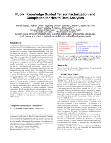
MedicationsCentral sympatholyticsAngiotensin receptor blockersACE inhibitorsImmunosuppressantsLoop diureticsGabapentin0.8AvgOverlapDiagnosesChronic kidney diseaseHypertensionUnspecified anemiasFluid electrolyte imbalanceType 2 diabetes mellitusOther kidney disordersTable 7: Examples of Rubik-derived subphenotypes.The two tables show separate subgroups of hypertension patients: A) metabolic syndrome, and B)secondary hypertension due to renovascular disease.out of 8) of all subphenotypes as clinically meaningful, andthe remaining 37.5% of subphenotypes to be possibly clinically meaningful. None of the subphenotypes were identified as not clinically meaningful. These results suggest thatRubik can be effective for discovering subphenotypes givenknowledge guided constraints on the disease mode.4.2.4More Distinct PhenotypesOne important objective of phenotyping is to discover distinct phenotypes. In this experiment, we show that addingpairwise constraints guidance reduces the overlap betweenphenotypes. We also fix λa 0 and change the weight ofpairwise constraint (λq ) to evaluate the sensitivity of Rubikto this constraint.We first define cosine similarities between two vectors xhx,yi. Then we use AvgOverlap toand y as cos(x, y) kxkkykmeasure the degree of overlapping between all phenotypepairs. This is defined as the average of the cosine similaritiesbetween all phenotype pairs in

EHR data are consistent with existing studies on the pop-ulation. Rubik is also much more computationally scalable compared to all baseline methods, with up to a 7-fold de-crease in running time over the baselines. Symbol Description Khatri-Rao product outer product element-wise product N number of modes R number of latent phenotypes X;O tensor .