![Introducing PARALLEL: Stata Module For Parallel Computing [draft]](/img/54/parallel.jpg)
Transcription
Introducing PARALLEL: Stata Module forParallel Computing [draft]George Vega Yon Research DepartmentChilean Pension SupervisorThis version September 26, 2012AbstractInspired in the R library “snow” and to be used in multicore CPUs,parallel implements parallel computing methods through an OS’s shellscripting (using Stata in batch mode) to accelerate computations. Bysplitting the dataset into a determined number of clusters this modulerepeats a task simultaneously over the data-clusters, allowing to increaseefficiency between two and five times, or more depending on the numberof cores of the CPU. Without the need of StataMP, parallel is, to theauthor’s knowledge, the first user contributed Stata module to implementparallel computing.Keywords: Parallel Computing, High Performance Computing, Simulation Methods, CPUJEL Codes: C87, C15, C61 gvegaat spensiones.cl. Thanks to Damian C. Clarke, Félix Villatoro and Eduardo Fajnzylber and the Research team of the Chilean Pension Supervisor for their valuable contributions.The usual disclaimers applies.1
1IntroductionCurrently home computers are arriving with extremely high computational capabilities. Multicore CPUs, standard in today’s industry, expand the boundaries of productivity for the so called multitasking-users. Motivated by thevideo games industry, manufacturers have forged a market for low-cost processing units with the number-crunching horsepower comparable to that of a smallsupercomputer (?, ?).In the same way, data availability has improved in a significant manner. BigData is an active topic by computer scientists and policy-makers considering thenumber of open-data initiatives taking place around the globe giving access toadministrative data. Resources that, despite being available to researchers andpolicy makers, have not been exploited as they should.The limited use of these social data resources is not a coincidence. As GaryKing states in ? (?), issues involving privacy, standardized management andlack of statistical computing tools are still unsolved both for social scientists,and policy-makers. parallel aims to make a contribution to these issues.2Parallel ComputingIn simple terms, parallel computing is the simultaneous use of multiple computeresources to solve a computational problem (?, ?). Parallelism can take placethrough several levels starting from (a) bit level, (b) instruction level, (c) datalevel and up to (d) task level. parallel uses data level parallelism, whichbasically consists in simultaneously repeating an instruction over independentgroups of data.Using parallel computing allows the user to drastically decrease the timerequired to complete a computational problem. This is especially important fordata scientists such as empirical economists and econometricians, given that inthis way it is possible to implement algorithms characterized by a large numberof calculations or, in the case of Stata, code interpretation such as flow-controlstatements like loops.Flynn’s taxonomy classification provides a simple way to classify the type ofparallelisms that researchers may require. Based on the type of instruction andthe type of data, both of which can be single or multiple, Flynn identifies fourclasses of computer architectures (?, ?).According to this classification, parallel would follow a Single Instruction2
Table 1: Flynn’s taxonomySingle Instruction Multiple InstructionSingle DataSISDMISDMultiple DataSIMDMIMDMultiple Data (SIMD) design, where the parallelism takes place by repeatinga single task over groups of data. Even though this is a very simple form ofparallelism, significant improvements can be achieved from its use.With regards to the size of the improvements, following Amdahl’s law,the speed improvement S depends upon (a) the proportion of potential deserialization P ; this is, the proportion of the algorithm that can be implementedin a parallel fashion, and (b) the number of fractions to be split, N .S 1(1 P ) PN(1)Thus, if P tends to one, the potential speed gains S will be equal to N .In the same way, as P approaches to zero, any parallelization attempt willbe worthless1 . Considering this, theoretically, SIMD class may reach perfectscaling.3Parallel Computing in EconometricsEven though parallel computing is not a new idea2 , economics has drawn relatively little from parallel computing. In ? (?) efforts are made by introducing anew C library based on matrix programming language Ox with the objective topromote parallel computing in social sciences. Using alternative approach, andafter experimenting with GPU based parallel computing, ? (?) show that usingthis approach to solve a Real Business Cycle model and using a consumer levelNVIDIA video card, it is possible to reach speed improvements of around twohundred times, with this being a lower bound.Statistical packages are also advancing in this line. Matlab provides its ownParallel Computing Toolbox3 which makes it possible to implement parallelcomputing methods through multicore computer, GPUs and computer clusters.1Agood technical review on modern themes on parallel computing is provided by ? (?)sciences, physics, computer science and industry have taken considerable advantage of it.3 ng/2 Applied3
GNU open-source R also has several libraries to implement parallel computingalgorithms such as parallel, snow, and so forth4 . And Stata with its MultiProcessor edition, StataMP, implementing bit level parallelization makes it possible to achieve up to (or greater than) constant scale speed improvements (?,?).4PARALLEL: Stata module for parallel computingInspired by the R library “snow” and to be used in multicore CPUs, parallelimplements parallel computing methods through OS’s shell scripting (usingStata in batch mode) to speedup computations by splitting the dataset intoa determined number of clusters5 in such a way to implement a data parallelismalgorithm.As exposed in Figure 1, right after parallel splits the dataset into n clustersit starts n new independent stata instances in batch mode over which the sametask is simultaneously executed. By default all the loaded instance globals and,optionally, programs and mata objects/programs are passed through. Afterevery cluster stops the resulting datasets are appended and returned to thecurrent stata instance without modifying other elements.4 For more details see CRAN Task View on High-Performance and Parallel ComputingWith R eComputing.html5 It is important to distinguish between two different ways to understand a cluster. Incomputer science a cluster, or computer cluster, refers to a set of computers connected so thatthey to work as a single system. Here, in the other hand, as this module is intended to be useby statisticians and social scientist in general, I refer to a cluster as a package of data whichin this case does not necessary contains related observations (clustered).4
Figure 1: How parallel rting (current) stata instance loadedwith data plus user defined globals,programs, mata objects and mataprogramsSplitting the data Task (stata batch-mode)Cluster1’Cluster2’Cluster3’.A new stata instance (batch-mode) forevery data-clusters. Programs, globals andmata objects/programs are passed to them.The same algorithm (task) is simultaneously applied over the data-clusters.Clustern’After every instance stops, the data-clustersare appended into one.Appending the data nding (resulting) stata instance loadedwith the new data.User defined globals, programs, mataobjects and mata programs remind unchanged.
The number of efficient computing clusters depends upon the number ofphysical cores (CPUs) with which your computer is built, e.g. if you have aquad-core computer, the correct cluster setting should be four. In the case ofsimultaneous multithreading, such as that from Intel’s hyper-threading technology (HTT), setting parallel following the number of processors threads,as it was expected, hardly results into a perfect speedup scaling. In spite ofit, after several tests on HTT capable architectures, the results of implementing parallel according to the machines physical cores versus its logicals showssmall though significant differences.parallel is especially handy when it comes to implementing loop-basedsimulation models (or simply loops), Stata commands such as reshape, or anyjob that (1) can be repeated through data-blocks, and (2) routines that processesbig datasets.In the case of (pseudo) random number generation, parallel allows to setone seed per cluster with the option seeds(numlist).At this time parallel has been successfully tested in Windows and Unixmachines. Tests using Mac OS are still pending.4.1Syntaxparallel’s simplistic syntax is one of its key features. In order to use it, only twocommands needed be entered: parallel setclusters, which tells parallelhow many blocks of data are to be built (and thus how many Stata batch modeinstances are needed to be run), and parallel do (to run a do-file in parallel)or parallel: (to use it as a prefix to parallelize a command). More, detailed,as specified in its help-file:Setting the number of clusters (blocks of data)parallel setclusters #Parallelizing a dofileparallel do filename [,options ]Parallelizing a stata commandparallel [, options ]:stata cmdRemoving auxiliary filesparallel clean [parallelid ]6
5ResultsIn what follows, I present some results testing the efficiency of parallel overdifferent hardware and software configurations using StataSE. The tables summarize the results. The first row presents the time required to complete thetask using a single processor (cluster or thread as a computer scientist mayprefer). The second line shows the total time spent to complete the task usingparallel, while the following three distinguish between setup (time taken toprepare the algorithm), compute (execution time of the task as such) and finish(mainly appending the datasets). Finally the last two show the ratio of CPUtime over compute and total time respectively. Every time measure is presentedin seconds.It is important to consider that both setup time and finishing time increasesas the problem size scales up.All the test were performed checking whether if the parallel implementationreturned different results from the serial implementation.5.1Serial replacing using a loopThis first test consists on, after a generation of N pseudo-random values, usingstata’s rnormal() function, replacing each and every one of the observationsin a serial way (loop) starting from 1 to N . The observation’s variable wasreplaced using the PDF of the normal distribution.1 x2f (x) e 22π(2)The code to be parallelized is--------------- begin of do-file ------------local size Nforval i 1/‘size’ {qui replace x 1/sqrt(2*‘c(pi)’)*exp(-(x 2/2)) in ‘i’}--------------- end of do-file ---------------which is contained inside a do-file named “myloop.do”, and can be executedthrough four clusters with parallel as it followsparallel setclusters 4parallel do myloop.do7
This algorithm was repeated overN {10, 000; 100, 000; 1, 000, 000; 10, 000, 000}Table 2: Serial replacing using a loop on a Windows Machine (2 clusters)Problem Size10.000 100.000 1.000.000 nish0.250.250.300.62Ratio (compute)0.231.011.651.78Ratio (total)0.150.801.471.61Tested on an Intel Core i5 M560 (dual-core) machineTable 3: Serial replacing using a loop on a Linux Server (4 clusters)Problem Size10.000 100.000 1.000.000 inish0.210.230.461.47Ratio (compute)1.132.684.574.90Ratio (total)0.561.793.434.13Tested on an Intel Xeon X470 (octa-core) machine8
5.2Reshaping a large databaseReshaping a large database is always a time consuming task. This exampleshows the execution of Stata’s reshape wide command for a large administrative dataset which contains unemployment insurance solicitations made by itsusers, i.e. a panel dataset.The task was repeated over different sample sizesN {1, 000; 10, 000; 100, 000; 1, 000, 000; 10, 000, 000}Using parallel prefix syntax, the command is as it followsparallel, by(numcue) force:reshape wide ///tipsolic rutemp opta derecho ngiros, i(numcue) j(tiempo)where the options by consider observations grouping in so as not to split inbetween and force, jointly used with by, tells parallel not to check whetherif the dataset is actually sorted by, in this case, numcue.Table 4: Reshaping wide a large database on a Windows Machine (2 clusters)Problem Size100000 1000000 Ratio (compute)1.141.371.41Ratio (total)0.981.211.25Tested on an Intel Core i5 M560 (dual-core) machine9
Table 5: Reshaping wide a large database on a Windows Machine (4 clusterswith HTT)Problem Size100000 1000000 1Ratio (compute)1.282.141.90Ratio (total)1.111.741.52Tested on an Intel Core i5 M560 (dual-core) machineTable 6: Reshaping wide a large database on a Linux Server (4 clusters)Problem Size100.000 1.000.000 9824.53Ratio (compute)2.842.651.99Ratio (total)2.042.321.78Tested on an Intel Xeon X470 (octa-core) machineTable 7: Reshaping wide a large database on a Linux Server (8 clusters)Problem Size100000 1000000 7.07Ratio (compute)3.742.462.84Ratio (total)2.332.102.28Tested on an Intel Xeon X470 (octa-core) machine5.3Extended test: Monte Carlo SimulationIn ? (?) a simple Monte Carlo experiment is perform which simulates theperformance of a estimator of sample mean, x̄, in a context of heteroskedasticity.10
The model to beyi µ i N (0, σ 2 )(3)Let be a N (0, 1) variable multiplied by a factor czi , where zi varies over i.We will vary parameter c between 0.1 and 1.0 and determine its effect on thepoint and interval estimates of µ; as a comparison, we will compute a secondrandom variable which is homoskedastic, with the scale factor equalling cz̄.From web dataset census2 the variables age, region (which can be 1, 2, 3or 4) and the mean of region are used as µ, zi and z̄ respectively.The simulation program, stored in “mcsimul1.ado”, is defined as--------------- begin of ado-file -----------program define mcsimul1, rclassversion 10.0syntax [, c(real 1)]tempvar e1 e2gen double ‘e1’ invnorm(uniform())*‘c’*zmugen double ‘e2’ invnorm(uniform())*‘c’*z factorreplace y1 true y ‘e1’replace y2 true y ‘e2’summ y1return scalar mu1 r(mean)return scalar se mu1 r(sd)/sqrt(r(N))summ y2return scalar mu2 r(mean)return scalar se mu2 r(sd)/sqrt(r(N))return scalar c ‘c’end--------------- end of ado-file --------------In what is next, the do-file that runs the simulation, stored as “montecarlo.do”, it is compound of two parts: (a) setting the iteration range by whichc is going to vary, and (b) looping over the selected range. For the first partthe do-file uses the local macro pll instance which is the numer of the parallelstata instance running, thus there are as many as clusters have been declared,11
number available with the global macro PLL CLUSTERS. This way, if the macroPLL CLUSTERS equals two and the macro pll instance equals une, then therange will be defined from one to five6 .--------------- begin of do-file ------------// Defining the loop rangelocal num of intervals 10if length("‘pll id’") 0 {local start 1local end ‘num of intervals’}else {local ntot floor(‘num of intervals’/ PLL CLUSTERS)local start (‘pll instance’ - 1)*‘ntot’ 1local end (‘pll instance’)*‘ntot’if ‘pll instance’ PLL CLUSTERS local end 10}local reps 1000// Loopforval i ‘start’/‘end’ {qui webuse census2, cleargen true y agegen z factor regionsum z factor, meanonlyscalar zmu r(mean)qui {gen y1 .gen y2 .local c ‘i’/10set seed ‘c’simulate c r(c) mu1 r(mu1) se mu1 r(se mu1) ///mu2 r(mu2) se mu2 r(se mu2), ///saving(cc‘i’, replace) nodots reps(‘reps’): ///mcsimul1, c(‘c’)}}--------------- end of do-file ---------------This do-file will be executed from stata using parallel do syntax. As there6 Note that if the local macro pll id, which contains a special random number that identifiesan specific parallel run (more details in its help file), length is zero it means that the do-fileis not running in parallel mode, thus it is been executed in a serial way where the loop rangestarts from one to ten.12
is no need of splitting any dataset (these are loaded every time that the mainloop simul.do’s loop runs), we add the option nodata. This way the main dofile will look like this Finally, the do-file from which parallel runs the simulation--------------- begin of do-file ------------clear allparallel setclusters 5parallel do loop simul.do, nodata--------------- end of do-file ---------------By this parallel will start, in this case, five new independent stata instances, each one looping over the ranges 1/2, 3/4, 5/6, 7/8 and 9/10 respectively.Most of the code has been exactly copied with the exception of the additionof a new code line set seed. In order to be able to compare both serial andparallel implementations of the algorithm it was necessary to set a particularseed for each loop, inside “montecarlo.do” right before simulate command.Table 8: Monte Carlo Experiment on a Windows MachineNumber of 2Compute17.2718.07Finish0.110.11Ratio (compute) 1.651.60Ratio (total)1.631.58Tested on a Intel Core i5 M560 (dual-core) machine13
Table 9: Monte Carlo Experiment on a Linux ServerNumber of Clusters235CPU40.97 39.0136.44Total18.35 15.207.62Setup0.110.110.12Compute18.13 14.997.41Finish0.100.100.10Ratio (compute) 2.262.604.92Ratio (total)2.232.574.78Tested on a Intel Xeon X470 (octa-core) machine6Concluding RemarksAs stated by computer scientist Ph.D. Wen-Mei Hwu7 , parallel computing isthe future of supercomputing, and giving the computer industry’s fast pace ofdevelopment, scientists in various areas are making real efforts to promote itsusage. In spite of this, many of social scientist do not work with it due to itslack of user-friendly implementations.In the case of Stata, parallel is, to the authors knowledge, the first publicuser-contribution to parallel computing. The major benefits, measured in termsof speedups, can be reached by simulation models and non-vectorized operationssuch as control-flow statements. Speed gains are directly related to the proportion of the algorithm that can be de-serialized and the number of processorswith which the parallelization is made, making possible reach near to constantscale improvements.Notwithstanding the simplicity of this type of parallelism, giving to its easyway, it seems like a worthy activity for a wide range of social scientists andresearchers.7 Chief Scientist at Parallel Computing Institute ath-future14
level and up to (d) task level. parallel uses data level parallelism, which basically consists in simultaneously repeating an instruction over independent groups of data. Using parallel computing allows the user to drastically decrease the time required to complete a computational problem. This is especially important for