Transcription
4Data-Level Parallelism inVector, SIMD, and GPUArchitecturesWe call these algorithms data parallel algorithms because their parallelismcomes from simultaneous operations across large sets of data, rather thanfrom multiple threads of control.W. Daniel Hillis and Guy L. Steele“Data Parallel Algorithms,” Comm. ACM (1986)If you were plowing a field, which would you rather use: two strongoxen or 1024 chickens?Seymour Cray, Father of the Supercomputer(arguing for two powerful vector processorsversus many simple processors)Computer Architecture. DOI: 10.1016/B978-0-12-383872-8.00005-7 2012 Elsevier, Inc. All rights reserved.1
262 Chapter Four Data-Level Parallelism in Vector, SIMD, and GPU Architectures4.1IntroductionA question for the single instruction, multiple data (SIMD) architecture, whichChapter 1 introduced, has always been just how wide a set of applications hassignificant data-level parallelism (DLP). Fifty years later, the answer is not onlythe matrix-oriented computations of scientific computing, but also the mediaoriented image and sound processing. Moreover, since a single instruction canlaunch many data operations, SIMD is potentially more energy efficient thanmultiple instruction multiple data (MIMD), which needs to fetch and executeone instruction per data operation. These two answers make SIMD attractive forPersonal Mobile Devices. Finally, perhaps the biggest advantage of SIMD versus MIMD is that the programmer continues to think sequentially yet achievesparallel speedup by having parallel data operations.This chapter covers three variations of SIMD: vector architectures, multimedia SIMD instruction set extensions, and graphics processing units (GPUs).1The first variation, which predates the other two by more than 30 years,means essentially pipelined execution of many data operations. These vectorarchitectures are easier to understand and to compile to than other SIMD variations, but they were considered too expensive for microprocessors until recently.Part of that expense was in transistors and part was in the cost of sufficientDRAM bandwidth, given the widespread reliance on caches to meet memoryperformance demands on conventional microprocessors.The second SIMD variation borrows the SIMD name to mean basically simultaneous parallel data operations and is found in most instruction set architecturestoday that support multimedia applications. For x86 architectures, the SIMDinstruction extensions started with the MMX (Multimedia Extensions) in 1996,which were followed by several SSE (Streaming SIMD Extensions) versions inthe next decade, and they continue to this day with AVX (Advanced VectorExtensions). To get the highest computation rate from an x86 computer, you oftenneed to use these SIMD instructions, especially for floating-point programs.The third variation on SIMD comes from the GPU community, offeringhigher potential performance than is found in traditional multicore computerstoday. While GPUs share features with vector architectures, they have their owndistinguishing characteristics, in part due to the ecosystem in which they evolved.This environment has a system processor and system memory in addition to theGPU and its graphics memory. In fact, to recognize those distinctions, the GPUcommunity refers to this type of architecture as heterogeneous.1This chapter is based on material in Appendix F, “Vector Processors,” by Krste Asanovic, and Appendix G, “Hardwareand Software for VLIW and EPIC” from the 4th edition of this book; on material in Appendix A, “Graphics and Computing GPUs,” by John Nickolls and David Kirk, from the 4th edition of Computer Organization and Design; and to alesser extent on material in “Embracing and Extending 20th-Century Instruction Set Architectures,” by Joe Gebis andDavid Patterson, IEEE Computer, April 2007.
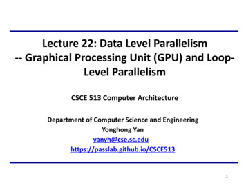
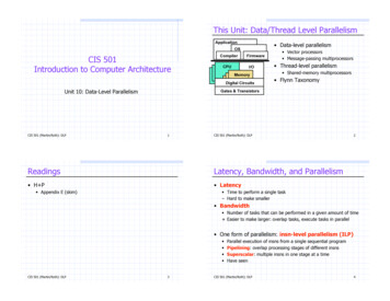
4.1Introduction 2631000MIMD*SIMD (32 b)MIMD*SIMD (64 b)SIMD (32 b)SIMD (64 b)Potential parallel speedupMIMD100101200320072011201520192023Figure 4.1 Potential speedup via parallelism from MIMD, SIMD, and both MIMD andSIMD over time for x86 computers. This figure assumes that two cores per chip forMIMD will be added every two years and the number of operations for SIMD will doubleevery four years.For problems with lots of data parallelism, all three SIMD variations sharethe advantage of being easier for the programmer than classic parallel MIMDprogramming. To put into perspective the importance of SIMD versus MIMD,Figure 4.1 plots the number of cores for MIMD versus the number of 32-bit and64-bit operations per clock cycle in SIMD mode for x86 computers over time.For x86 computers, we expect to see two additional cores per chip every twoyears and the SIMD width to double every four years. Given these assumptions,over the next decade the potential speedup from SIMD parallelism is twice that ofMIMD parallelism. Hence, it’s as least as important to understand SIMD parallelism as MIMD parallelism, although the latter has received much more fanfarerecently. For applications with both data-level parallelism and thread-level parallelism, the potential speedup in 2020 will be an order of magnitude higher than today.The goal of this chapter is for architects to understand why vector is moregeneral than multimedia SIMD, as well as the similarities and differencesbetween vector and GPU architectures. Since vector architectures are supersetsof the multimedia SIMD instructions, including a better model for compilation,and since GPUs share several similarities with vector architectures, we start with
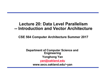
264 Chapter Four Data-Level Parallelism in Vector, SIMD, and GPU Architecturesvector architectures to set the foundation for the following two sections. The nextsection introduces vector architectures, while Appendix G goes much deeper intothe subject.4.2Vector ArchitectureThe most efficient way to execute a vectorizable application is a vectorprocessor.Jim SmithInternational Symposium on Computer Architecture (1994)Vector architectures grab sets of data elements scattered about memory, placethem into large, sequential register files, operate on data in those register files,and then disperse the results back into memory. A single instruction operates onvectors of data, which results in dozens of register–register operations on independent data elements.These large register files act as compiler-controlled buffers, both to hidememory latency and to leverage memory bandwidth. Since vector loads andstores are deeply pipelined, the program pays the long memory latency only onceper vector load or store versus once per element, thus amortizing the latencyover, say, 64 elements. Indeed, vector programs strive to keep memory busy.VMIPSWe begin with a vector processor consisting of the primary components thatFigure 4.2 shows. This processor, which is loosely based on the Cray-1, is thefoundation for discussion throughout this section. We will call this instructionset architecture VMIPS; its scalar portion is MIPS, and its vector portion is thelogical vector extension of MIPS. The rest of this subsection examines how thebasic architecture of VMIPS relates to other processors.The primary components of the instruction set architecture of VMIPS are thefollowing: Vector registers—Each vector register is a fixed-length bank holding a singlevector. VMIPS has eight vector registers, and each vector register holds 64 elements, each 64 bits wide. The vector register file needs to provide enough portsto feed all the vector functional units. These ports will allow a high degree ofoverlap among vector operations to different vector registers. The read andwrite ports, which total at least 16 read ports and 8 write ports, are connected tothe functional unit inputs or outputs by a pair of crossbar switches. Vector functional units—Each unit is fully pipelined, and it can start a newoperation on every clock cycle. A control unit is needed to detect hazards,both structural hazards for functional units and data hazards on registeraccesses. Figure 4.2 shows that VMIPS has five functional units. For simplicity, we focus exclusively on the floating-point functional units.
4.2Vector Architecture 265Main memoryVectorload/storeFP add/subtractFP multiplyFP Figure 4.2 The basic structure of a vector architecture, VMIPS. This processor has ascalar architecture just like MIPS. There are also eight 64-element vector registers, andall the functional units are vector functional units. This chapter defines special vectorinstructions for both arithmetic and memory accesses. The figure shows vector units forlogical and integer operations so that VMIPS looks like a standard vector processor thatusually includes these units; however, we will not be discussing these units. The vectorand scalar registers have a significant number of read and write ports to allow multiplesimultaneous vector operations. A set of crossbar switches (thick gray lines) connectsthese ports to the inputs and outputs of the vector functional units. Vector load/store unit—The vector memory unit loads or stores a vector to orfrom memory. The VMIPS vector loads and stores are fully pipelined, so thatwords can be moved between the vector registers and memory with a bandwidth of one word per clock cycle, after an initial latency. This unit wouldalso normally handle scalar loads and stores. A set of scalar registers—Scalar registers can also provide data as input tothe vector functional units, as well as compute addresses to pass to the vectorload/store unit. These are the normal 32 general-purpose registers and 32floating-point registers of MIPS. One input of the vector functional unitslatches scalar values as they are read out of the scalar register file.
266 Chapter Four Data-Level Parallelism in Vector, SIMD, and GPU VS.DV1,V2,V3V1,V2,F0Add elements of V2 and V3, then put each result in V1.Add F0 to each element of V2, then put each result in btract elements of V3 from V2, then put each result in V1.Subtract F0 from elements of V2, then put each result in V1.Subtract elements of V2 from F0, then put each result in V1.MULVV.DMULVS.DV1,V2,V3V1,V2,F0Multiply elements of V2 and V3, then put each result in V1.Multiply each element of V2 by F0, then put each result in vide elements of V2 by V3, then put each result in V1.Divide elements of V2 by F0, then put each result in V1.Divide F0 by elements of V2, then put each result in V1.LVV1,R1Load vector register V1 from memory starting at address R1.SVR1,V1Store vector register V1 into memory starting at address R1.LVWSV1,(R1,R2)Load V1 from address at R1 with stride in R2 (i.e., R1 i R2).SVWS(R1,R2),V1Store V1 to address at R1 with stride in R2 (i.e., R1 i R2).LVIV1,(R1 V2)Load V1 with vector whose elements are at R1 V2(i) ( i.e., V2 is an index).SVI(R1 V2),V1Store V1 to vector whose elements are at R1 V2(i) (i.e., V2 is an index).CVIV1,R1Create an index vector by storing the values 0, 1 R1, 2 R1,.,63 R1 into V1.S--VV.DS--VS.DV1,V2V1,F0Compare the elements (EQ, NE, GT, LT, GE, LE) in V1 and V2. If condition is true, put a1 in the corresponding bit vector; otherwise put 0. Put resulting bit vector in vectormask register (VM). The instruction S--VS.D performs the same compare but using ascalar value as one operand.POPR1,VMCount the 1s in vector-mask register VM and store count in R1.CVMSet the vector-mask register to all 1s.MTC1MFC1VLR,R1R1,VLRMove contents of R1 to vector-length register VL.Move the contents of vector-length register VL to R1.MVTMMVFMVM,F0F0,VMMove contents of F0 to vector-mask register VM.Move contents of vector-mask register VM to F0.Figure 4.3 The VMIPS vector instructions, showing only the double-precision floating-point operations. Inaddition to the vector registers, there are two special registers, VLR and VM, discussed below. These special registersare assumed to live in the MIPS coprocessor 1 space along with the FPU registers. The operations with stride anduses of the index creation and indexed load/store operations are explained later.Figure 4.3 lists the VMIPS vector instructions. In VMIPS, vector operationsuse the same names as scalar MIPS instructions, but with the letters “VV”appended. Thus, ADDVV.D is an addition of two double-precision vectors. Thevector instructions take as their input either a pair of vector registers (ADDVV.D)or a vector register and a scalar register, designated by appending “VS”(ADDVS.D). In the latter case, all operations use the same value in the scalar register as one input: The operation ADDVS.D will add the contents of a scalar registerto each element in a vector register. The vector functional unit gets a copy of thescalar value at issue time. Most vector operations have a vector destination register, although a few (such as population count) produce a scalar value, which isstored to a scalar register.
4.2Vector Architecture 267The names LV and SV denote vector load and vector store, and they load orstore an entire vector of double-precision data. One operand is the vector register to be loaded or stored; the other operand, which is a MIPS general-purposeregister, is the starting address of the vector in memory. As we shall see, in addition to the vector registers, we need two additional special-purpose registers: thevector-length and vector-mask registers. The former is used when the naturalvector length is not 64 and the latter is used when loops involve IF statements.The power wall leads architects to value architectures that can deliver highperformance without the energy and design complexity costs of highly outof-order superscalar processors. Vector instructions are a natural match to thistrend, since architects can use them to increase performance of simple in-orderscalar processors without greatly increasing energy demands and design complexity. In practice, developers can express many of the programs that ran wellon complex out-of-order designs more efficiently as data-level parallelism in theform of vector instructions, as Kozyrakis and Patterson [2002] showed.With a vector instruction, the system can perform the operations on the vectordata elements in many ways, including operating on many elements simultaneously. This flexibility lets vector designs use slow but wide execution units toachieve high performance at low power. Further, the independence of elementswithin a vector instruction set allows scaling of functional units without performing additional costly dependency checks, as superscalar processors require.Vectors naturally accommodate varying data sizes. Hence, one view of avector register size is 64 64-bit data elements, but 128 32-bit elements, 256 16-bitelements, and even 512 8-bit elements are equally valid views. Such hardwaremultiplicity is why a vector architecture can be useful for multimedia applications as well as scientific applications.How Vector Processors Work: An ExampleWe can best understand a vector processor by looking at a vector loop for VMIPS.Let’s take a typical vector problem, which we use throughout this section:Y a X YX and Y are vectors, initially resident in memory, and a is a scalar. This problemis the so-called SAXPY or DAXPY loop that forms the inner loop of the Linpackbenchmark. (SAXPY stands for single-precision a X plus Y; DAXPY for double precision a X plus Y.) Linpack is a collection of linear algebra routines, andthe Linpack benchmark consists of routines for performing Gaussian elimination.For now, let us assume that the number of elements, or length, of a vectorregister (64) matches the length of the vector operation we are interested in. (Thisrestriction will be lifted shortly.)ExampleAnswerShow the code for MIPS and VMIPS for the DAXPY loop. Assume that the starting addresses of X and Y are in Rx and Ry, respectively.Here is the MIPS code.
268 Chapter Four Data-Level Parallelism in Vector, SIMD, and GPU Loop;load scalar a;last address to load;load X[i];a X[i];load Y[i];a X[i] Y[i];store into Y[i];increment index to X;increment index to Y;compute bound;check if doneHere is the VMIPS code for yV4,V2,V3V4,Ry;load scalar a;load vector X;vector-scalar multiply;load vector Y;add;store the resultThe most dramatic difference is that the vector processor greatly reduces thedynamic instruction bandwidth, executing only 6 instructions versus almost600 for MIPS. This reduction occurs because the vector operations work on 64elements and the overhead instructions that constitute nearly half the loop onMIPS are not present in the VMIPS code. When the compiler produces vectorinstructions for such a sequence and the resulting code spends much of its timerunning in vector mode, the code is said to be vectorized or vectorizable. Loopscan be vectorized when they do not have dependences between iterations of aloop, which are called loop-carried dependences (see Section 4.5).Another important difference between MIPS and VMIPS is the frequency ofpipeline interlocks. In the straightforward MIPS code, every ADD.D must wait fora MUL.D, and every S.D must wait for the ADD.D. On the vector processor, eachvector instruction will only stall for the first element in each vector, and then subsequent elements will flow smoothly down the pipeline. Thus, pipeline stalls arerequired only once per vector instruction, rather than once per vector element.Vector architects call forwarding of element-dependent operations chaining, inthat the dependent operations are “chained” together. In this example, thepipeline stall frequency on MIPS will be about 64 higher than it is on VMIPS.Software pipelining or loop unrolling (Appendix H) can reduce the pipeline stallson MIPS; however, the large difference in instruction bandwidth cannot bereduced substantially.Vector Execution TimeThe execution time of a sequence of vector operations primarily depends on threefactors: (1) the length of the operand vectors, (2) structural hazards among the
4.2Vector Architecture 269operations, and (3) the data dependences. Given the vector length and the initiation rate, which is the rate at which a vector unit consumes new operands andproduces new results, we can compute the time for a single vector instruction. Allmodern vector computers have vector functional units with multiple parallelpipelines (or lanes) that can produce two or more results per clock cycle, but theymay also have some functional units that are not fully pipelined. For simplicity,our VMIPS implementation has one lane with an initiation rate of one elementper clock cycle for individual operations. Thus, the execution time in clockcycles for a single vector instruction is approximately the vector length.To simplify the discussion of vector execution and vector performance, weuse the notion of a convoy, which is the set of vector instructions that couldpotentially execute together. As we shall soon see, you can estimate performanceof a section of code by counting the number of convoys. The instructions in aconvoy must not contain any structural hazards; if such hazards were present, theinstructions would need to be serialized and initiated in different convoys. Tokeep the analysis simple, we assume that a convoy of instructions must completeexecution before any other instructions (scalar or vector) can begin execution.It might seem that in addition to vector instruction sequences with structuralhazards, sequences with read-after-write dependency hazards should also be inseparate convoys, but chaining allows them to be in the same convoy.Chaining allows a vector operation to start as soon as the individual elementsof its vector source operand become available: The results from the first functional unit in the chain are “forwarded” to the second functional unit. In practice,we often implement chaining by allowing the processor to read and write a particular vector register at the same time, albeit to different elements. Early implementations of chaining worked just like forwarding in scalar pipelining, but thisrestricted the timing of the source and destination instructions in the chain.Recent implementations use flexible chaining, which allows a vector instructionto chain to essentially any other active vector instruction, assuming that we don’tgenerate a structural hazard. All modern vector architectures support flexiblechaining, which we assume in this chapter.To turn convoys into execution time we need a timing metric to estimate thetime for a convoy. It is called a chime, which is simply the unit of time taken toexecute one convoy. Thus, a vector sequence that consists of m convoys executesin m chimes; for a vector length of n, for VMIPS this is approximately m nclock cycles. The chime approximation ignores some processor-specific overheads, many of which are dependent on vector length. Hence, measuring time inchimes is a better approximation for long vectors than for short ones. We will usethe chime measurement, rather than clock cycles per result, to indicate explicitlythat we are ignoring certain overheads.If we know the number of convoys in a vector sequence, we know the execution time in chimes. One source of overhead ignored in measuring chimes is anylimitation on initiating multiple vector instructions in a single clock cycle. If onlyone vector instruction can be initiated in a clock cycle (the reality in most vectorprocessors), the chime count will underestimate the actual execution time of a
270 Chapter Four Data-Level Parallelism in Vector, SIMD, and GPU Architecturesconvoy. Because the length of vectors is typically much greater than the numberof instructions in the convoy, we will simply assume that the convoy executes inone chime.ExampleShow how the following code sequence lays out in convoys, assuming a singlecopy of each vector functional 3V4,Ry;load vector X;vector-scalar multiply;load vector Y;add two vectors;store the sumHow many chimes will this vector sequence take? How many cycles per FLOP(floating-point operation) are needed, ignoring vector instruction issue overhead?AnswerThe first convoy starts with the first LV instruction. The MULVS.D is dependent onthe first LV, but chaining allows it to be in the same convoy.The second LV instruction must be in a separate convoy since there is a structural hazard on the load/store unit for the prior LV instruction. The ADDVV.D isdependent on the second LV, but it can again be in the same convoy via chaining.Finally, the SV has a structural hazard on the LV in the second convoy, so it mustgo in the third convoy. This analysis leads to the following layout of vectorinstructions into convoys:1. LVMULVS.D2. LVADDVV.D3. SVThe sequence requires three convoys. Since the sequence takes three chimes andthere are two floating-point operations per result, the number of cycles per FLOPis 1.5 (ignoring any vector instruction issue overhead). Note that, although weallow the LV and MULVS.D both to execute in the first convoy, most vectormachines will take two clock cycles to initiate the instructions.This example shows that the chime approximation is reasonably accurate forlong vectors. For example, for 64-element vectors, the time in chimes is 3, so thesequence would take about 64 3 or 192 clock cycles. The overhead of issuingconvoys in two separate clock cycles would be small.Another source of overhead is far more significant than the issue limitation.The most important source of overhead ignored by the chime model is vectorstart-up time. The start-up time is principally determined by the pipelininglatency of the vector functional unit. For VMIPS, we will use the same pipelinedepths as the Cray-1, although latencies in more modern processors have tendedto increase, especially for vector loads. All functional units are fully pipelined.
4.2Vector Architecture 271The pipeline depths are 6 clock cycles for floating-point add, 7 for floating-pointmultiply, 20 for floating-point divide, and 12 for vector load.Given these vector basics, the next several subsections will give optimizations that either improve the performance or increase the types of programs thatcan run well on vector architectures. In particular, they will answer the questions: How can a vector processor execute a single vector faster than one elementper clock cycle? Multiple elements per clock cycle improve performance. How does a vector processor handle programs where the vector lengths arenot the same as the length of the vector register (64 for VMIPS)? Since mostapplication vectors don’t match the architecture vector length, we need anefficient solution to this common case. What happens when there is an IF statement inside the code to be vectorized?More code can vectorize if we can efficiently handle conditional statements. What does a vector processor need from the memory system? Without sufficient memory bandwidth, vector execution can be futile. How does a vector processor handle multiple dimensional matrices? Thispopular data structure must vectorize for vector architectures to do well. How does a vector processor handle sparse matrices? This popular data structure must vectorize also. How do you program a vector computer? Architectural innovations that are amismatch to compiler technology may not get widespread use.The rest of this section introduces each of these optimizations of the vector architecture, and Appendix G goes into greater depth.Multiple Lanes: Beyond One Element per Clock CycleA critical advantage of a vector instruction set is that it allows software to pass alarge amount of parallel work to hardware using only a single short instruction.A single vector instruction can include scores of independent operations yet beencoded in the same number of bits as a conventional scalar instruction. The parallel semantics of a vector instruction allow an implementation to execute theseelemental operations using a deeply pipelined functional unit, as in the VMIPSimplementation we’ve studied so far; an array of parallel functional units; or acombination of parallel and pipelined functional units. Figure 4.4 illustrates howto improve vector performance by using parallel pipelines to execute a vector addinstruction.The VMIPS instruction set has the property that all vector arithmetic instructions only allow element N of one vector register to take part in operations withelement N from other vector registers. This dramatically simplifies the construction of a highly parallel vector unit, which can be structured as multiple parallellanes. As with a traffic highway, we can increase the peak throughput of a vectorunit by adding more lanes. Figure 4.5 shows the structure of a four-lane vector
272 Chapter Four Data-Level Parallelism in Vector, SIMD, and GPU ArchitecturesElement group(a)(b)Figure 4.4 Using multiple functional units to improve the performance of a single vector add instruction,C A B. The vector processor (a) on the left has a single add pipeline and can complete one addition per cycle. Thevector processor (b) on the right has four add pipelines and can complete four additions per cycle. The elementswithin a single vector add instruction are interleaved across the four pipelines. The set of elements that movethrough the pipelines together is termed an element group. (Reproduced with permission from Asanovic [1998].)unit. Thus, going to four lanes from one lane reduces the number of clocks for achime from 64 to 16. For multiple lanes to be advantageous, both the applicationsand the architecture must support long vectors; otherwise, they will execute soquickly that you’ll run out of instruction bandwidth, requiring ILP techniques(see Chapter 3) to supply enough vector instructions.Each lane contains one portion of the vector register file and one executionpipeline from each vector functional unit. Each vector functional unit executesvector instructions at the rate of one element group per cycle using multiple pipelines, one per lane. The first lane holds the first element (element 0) for all vectorregisters, and so the first element in any vector instruction will have its source
4.2Lane 0FP addpipe 0Vectorregisters:elements0, 4, 8, . . .FP mul.pipe 0Lane 1Vector ArchitectureLane 2 Lane 3FP addpipe 1FP addpipe 2FP addpipe 3Vectorregisters:elements1, 5, 9, . . .Vectorregisters:elements2, 6, 10, . . .Vectorregisters:elements3, 7, 11, . . .FP mul.pipe 2FP mul.pipe 3FP mul.pipe 1273Vector load-store unitFigure 4.5 Structure of a vector unit containing four lanes. The vector register storage is divided across the lanes, with each lane holding every fourth element of eachvector register. The figure shows three vector functional units: an FP add, an FP multiply, and a load-store unit. Each of the vector arithmetic units contains four executionpipelines, one per lane, which act in concert to complete a single vector instruction.Note how each section of the vector register file only needs to provide enough portsfor pipelines local to its lane. This figure does not show the path to provide the scalaroperand for vector-scalar instructions, but the scalar processor (or control processor)broadcasts a scalar value to all lanes.and destination operands located in the first lane. This allocation allows the arithmetic pipeline local to the lane to complete the operation without communicatingwith other lanes. Accessing main memory also requires only intralane wiring.Avoiding interlane communication reduces the wiring cost and register file portsrequired to build a highly parallel execution unit, and helps explain why vectorcomputers can complete
significant data-level parallelism (DLP). Fifty years later, the answer is not only the matrix-oriented computations of scientific computing, but also the media-oriented image and sound processing. Moreover, since a single instruction can launch many data operations, SIMD is potentially more energy efficient than