Transcription
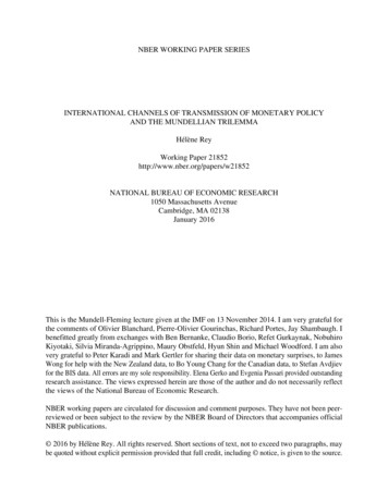
Jonathan McCarthy and Richard W. PeachMonetary PolicyTransmission to ResidentialInvestmentIntroductionThe volatility of residential investment has declinedconsiderably since the mid-1980s (Chart 1). The timing ofthis reduction in volatility corresponds to the timing of afundamental restructuring of the housing finance system, froma heavily regulated system dominated by thrift institutions(savings and loans and mutual savings banks) to a relativelyunregulated system dominated by mortgage bankers andbrokers and the process of mortgage securitization. With thisrestructuring, the housing finance system is now integratedwith the broader capital markets in the sense that “mortgagerates move in response to changes in other capital market rates,and mortgage funds are readily available at going market rates”(Hendershott and Van Order 1989).In light of this restructuring, it is certainly possible that thetransmission of monetary policy to residential investment haschanged. The supply of mortgage credit is now less likely toexperience the sharp swings that occurred in the 1960s and1970s. This, along with much greater competitiveness in theprimary mortgage market prompted by deregulation, suggeststhat a tightening of monetary policy is less likely to result innonprice rationing of mortgage credit, as was frequently thecase under the old system. Our goal in this paper is todocument any differences between the effects of changes inmonetary policy on residential investment under the currentand previous housing finance regimes.Jonathan McCarthy is an economist and Richard W. Peach a vice presidentat the Federal Reserve Bank of New York. jonathan.mccarthy@ny.frb.org richard.peach@ny.frb.org In the first half of the paper, we review the significantchanges in the housing finance system over the past thirty yearsand discuss the implications of these changes for the cost andavailability of mortgage credit. In the second half, we present atwo-part econometric analysis of the transmission of changesin monetary policy to residential investment. The first part usesa small, reduced-form macroeconomic model to examine theresponse of the housing market to a monetary policy “shock.”We then use a structural model of investment in single-familyhousing to examine the effect that the changes in the housingfinance system have had on the housing market and on theresponse of that market to changes in monetary policy. Ourmain conclusion is that the eventual magnitude of the responseof residential investment to a given change in monetary policyis similar to what it has been in the past. However, thatresponse does not occur as quickly as it did under the oldhousing finance system and its timing is now similar to that ofthe overall economy.Evolution of the HousingFinance SystemThe housing finance system can be thought of as threeinterrelated but distinct markets: the primary mortgagemarket, the secondary mortgage market, and the market forThe authors thank their discussant, Christopher Mayer, as well as Ken Kuttner,Trish Mosser, Jean Boivin, an anonymous referee, and the conferenceparticipants for comments, and Lauren Munyan and Don Rissmiller forresearch assistance. The views expressed are those of the authors and do notnecessarily reflect the position of the Federal Reserve Bank of New York orthe Federal Reserve System.FRBNY Economic Policy Review / May 2002139
Chart 1Residential Investment: Single-Family StructuresBillions of 1996 Chain-Weighted DollarsYear-over-year percentage change806040200-20-4019606570758085909500Sources: Bureau of Economic Analysis; Board of Governors of theFederal Reserve System, Flow of Funds.Note: Shaded regions indicate periods of deposit outflows.mortgage-backed securities (MBSs). Over the past thirty years,the underlying institutional setting of those markets has changeddramatically in response to macroeconomic conditions,deregulation, and financial and technological innovation. Thissection reviews those changes and discusses their implicationsfor the cost and availability of mortgage credit.Trends in the Primary Mortgage MarketThe primary mortgage market is where homeowners(mortgagors) borrow from mortgage lenders (originators),pledging their home as collateral for the debt. The debtinstrument created in this transaction is typically referred toas a whole loan. Thirty years ago, the primary market wasdominated by the heavily regulated thrift industry. Today, itis dominated by the relatively unregulated mortgagebanking industry.As recently as the 1970s, the primary mortgage market hadessentially the same structure as the one created during the1930s, often referred to as the New Deal system.1 Under thatsystem, thrifts gathered primarily local time deposits andmade long-term fixed-rate mortgage loans on residentialproperties located near their home offices,2 which were thenheld in the thrift’s portfolio. To enable thrifts to attract moreeasily the funds needed for mortgage lending, Regulation Q,which established maximum interest rates on deposits, gavethrifts a ceiling 25 basis points higher than the one for140Monetary Policy Transmission to Residential Investmentcommercial banks. Although thrifts were subject torestrictions on the assets they could acquire—no corporateloans, bonds, or equities—they benefited from a unique taxprovision that made it very profitable for them to invest inresidential mortgages.3This system was established for a variety of motives,including the promotion of home ownership and stableeconomic growth. It was also dictated to a large extent by thenature of the mortgage asset. Mortgages are promises to paymade by individuals, with their properties serving as collateral.Assessment of credit risk requires substantial knowledge oflocal market conditions, making individual mortgagesrelatively illiquid.The New Deal housing finance system worked quite well inthe relatively low-inflation environment of the 1950s and early1960s. However, by the late 1960s, as inflation began toincrease, the weaknesses of this system became evident. Thriftsfunded their portfolios of primarily long-term mortgage assetswith primarily short-term savings deposits. As interest ratesincreased, thrifts’ cost of funds rose quickly while the rate ofreturn on their portfolio of mortgages rose very slowly, sharplyreducing their net income. Moreover, as short-term interestrates rose above the Regulation Q ceilings, those short-termdeposits often flowed out of thrifts and commercial banks tohigher yielding alternatives, such as the newly emerging moneymarket mutual funds. As a consequence, these institutionswere forced to contract the flow of mortgage credit sharply,leading to steep contractions of residential construction andsales of existing homes. In addition to this interest rate risk, thegeographic limits placed on thrifts exposed them to substantialcredit risk during regional downturns. Finally, as thrifts wentfrom profitability to losses, the value of their loan loss taxprovision fell to zero.4The declining earnings of thrifts and these episodes ofdisintermediation led to two major policy thrusts. One was toexpand thrifts’ asset and liability powers to bolster theirearnings and preserve them as lending institutions with a focuson housing finance.5 The second was to foster the developmentof a market for mortgage-backed securities to enhance thrifts’liquidity and broaden the investor base for home mortgages,which we discuss in the next section. At the time, these effortsmay have been viewed as complementary. With hindsight,however, it is clear that the rapid growth of the market formortgage-backed securities contributed greatly to the loss ofthrifts’ cost advantages and thus to their declining importancein housing finance.Indeed, in the 1970s, thrifts originated 55 percent of longterm mortgages on one-to-four-family properties (Chart 2). Atthat time, mortgage companies or bankers tended to specializein loans insured by the Federal Housing Administration (FHA)
and loans guaranteed by the Department of Veterans Affairs(VA). This specialization limited their primary market share tojust 19 percent. Unlike thrifts, mortgage bankers are notdepository institutions. They fund mortgages through assortedforms of short-term borrowing—sometimes referred to as awarehouse line of credit—and then sell the loans for cash or“swap” them for mortgage-backed securities in the secondarymortgage market.6 By the mid-1990s, mortgage bankers andthrifts had switched roles, with mortgage bankers originating63 percent of loans closed over 1995-96 and thrifts originatingjust 19 percent.7 The rise of mortgage banking in the primarymarket was largely dependent upon changes in the secondarymortgage market and the development of the market for MBSs.Trends in the Secondary Mortgage MarketThe secondary mortgage market involves the sale and purchaseof whole loans originated in the primary market. Here, as in theprimary market, the role of thrift institutions has changedmarkedly over the past thirty years. In the 1970s, thrifts’ netacquisitions of mortgages exceeded their originations, indicatingthat thrifts were net purchasers of mortgages in the secondarymarket.8 However, after 1980, thrifts became net sellers ofmortgages, like commercial banks and mortgage bankers.The counterpart to thrifts becoming net sellers of mortgagesas well as the increasing market share of mortgage bankers inthe primary market has been the growth of the government-sponsored mortgage pools and, more recently, private conduitsas net acquirers of mortgages in the secondary market. Theseacquisitions then serve as the collateral for mortgage-backedsecurities, which entitle the holder to a portion of the cash flowgenerated by a pool of mortgage loans. The governmentsponsored mortgage pools are the Government NationalMortgage Association (GNMA, or Ginnie Mae), the FederalNational Mortgage Association (FNMA, or Fannie Mae), andthe Federal Home Loan Mortgage Corporation (FHLMC, orFreddie Mac).9 In addition to issuing MBSs, Fannie Mae andFreddie Mac, which are government-sponsored enterprises(GSEs) or federal credit agencies, have issued debt and acquiredsubstantial portfolios of mortgage loans (and MBSs).10Chart 3 presents the net acquisitions of the governmentsponsored mortgage pools, the federal credit agencies, andprivate conduits as shares of total single-family loanoriginations from 1970 to the late 1990s. In the early 1970s, thegovernment-sponsored pools acquired just 5 percent of totaloriginations. In the 1990s, their purchases averaged around50 percent of total originations.11 Private conduits did notexist in the early 1980s, but by the late 1990s they wereacquiring 5 percent of total originations. Also by the late 1990s,the federal credit agencies were purchasing 10 to 15 percent ofthe flow of originations to hold in their portfolios. Collectively,the government-sponsored pools, the federal credit agencies,and the private conduits were net purchasers of about twothirds of single-family originations during the late 1990s.This tremendous growth is a testament to the advantagesprovided by mortgage securitization, a process that began inChart 2Chart 3Market Shares of Long-Term Loan Originationsfor Single-Family PropertiesRatio of Net Acquisitions to Total Originationsfor Long-Term Single-Family LoansMarket share, percentage of total70MortgagecompaniesThrifts60500.7Mortgage pools0.60.540Commercialbanks30200.40.3Federal creditagenciesPrivate mortgage-backedsecurities 95Source: Housing and Urban Development Agency, Office of FinancialManagement, Survey of Mortgage Lending Activity.Source: Housing and Urban Development Agency, Office of FinancialManagement, Survey of Mortgage Lending Activity.Note: Figures are based on quarterly averages of monthly survey data.Note: Figures are based on quarterly averages of monthly survey data.FRBNY Economic Policy Review / May 2002141
earnest when Ginnie Mae issued the first mortgage pass-throughsecurity in 1970 and Freddie Mac began issuing mortgageparticipation certificates backed by conventional mortgage loansin 1971.12 Mortgage securitization is a way of overcoming theinherent illiquidity of whole mortgage loans. By poolingindividual mortgages, it is possible to diversify credit risk over alarge number of geographically dispersed borrowers andproperties. With diversification, credit risk could be more easilyevaluated, allowing the security issuer to add creditenhancement. For example, Ginnie Mae, Fannie Mae, andFreddie Mac mortgage-backed securities guarantee payment ofinterest and principal, freeing the investor from credit risk,although the investor is still subject to prepayment risk.13In addition to the diversification benefits derived frompooling mortgages, several other key factors spurred thegrowth of securitization. Because of the advantages conferredby their GSE status, Fannie Mae and Freddie Mac gained asignificant cost advantage over thrifts.14 The GSE advantagesinclude the market perception of a Treasury guarantee of thesecurities and debt that the agencies issue; the “qualifiedinvestment” status of the agencies’ debt for regulated financialinstitutions; and exemption from state and local taxes,Securities and Exchange Commission registration fees andrequirements, and many state securities laws. In addition,FIRREA lowered thrifts’ capital requirements for mortgagebacked securities relative to whole loans, increasing theirincentive to hold MBSs. Finally, new financial products furtherenlarged the investor pool for MBSs. For example, in 1983,Freddie Mac issued the first collateralized mortgage obligation(CMO), which divides the cash flow of a pool of mortgages intovarious maturity tranches, simultaneously creating short-termsecurities backed by mortgages and addressing the prepaymentrisk faced by investors in traditional MBSs.15Some private firms—private conduits—have begunsecuritizing mortgages, but they are limited primarily tononconforming conventional loans.16 Private securitizerscurrently cannot compete with Fannie Mae and Freddie Mac inthe conforming loan market because they must maintain morecapital, their securitization costs are higher, and they do nothave the economies of scale already realized by the GSEs.Since 1980, thrifts’ holdings of whole loans and MBSs havedeclined from more than 50 percent of the stock of homemortgage debt to around 13 percent by early 2000. In contrast,the share of home mortgage debt held by the federally relatedmortgage pools has risen from essentially zero in 1970 to10 percent in 1980, to 36 percent in 1990, and to 46 percent by2000. The holdings of the GSEs and the private asset-backedsecurities issuers have also risen rapidly, particularly in the 1990s.Implications for the Cost and Availabilityof Mortgage CreditWith the development of the modern housing finance system,the primary mortgage market has become fully integrated withthe capital markets. Consequently, the supply of mortgagecredit is no longer subject to sharp swings in availability relatedto the fortunes of thrifts in securing deposits. Rather, mortgagecredit is generally available at the going interest rate. Thischange is evident when comparing the growth of single-familyresidential investment with the rate of growth of thrift deposits.As seen in Chart 1, through the mid-1980s, periods of depositoutflows were associated with sharp declines in residentialinvestment. After the mid-1980s, that relationship no longerexisted. Also confirming the declining influence of thriftdeposit flows, Bradley, Gabriel, and Wohar (1995) find thatover the 1972-82 period, thrift provision of mortgage credithad a significant influence on the spread between mortgageinterest rates and yields on comparable-maturity Treasuries.However, as the housing finance system evolved, the authorsChart 4Shares of Outstanding Mortgage Debt by HolderPercent6050Savings institutions40Commercialbanks30Trends in Holdings of Mortgage DebtCorresponding to the changes in the primary and secondarymortgage markets, the past thirty years have also witnesseddramatic changes in holdings of home mortgage debt. Chart 4presents data on holdings of whole mortgage loans combinedwith our estimates of holdings of mortgage-backed securities.17142Monetary Policy Transmission to Residential Investment2010Asset-backedsecurities issuersRest of 5Source: Board of Governors of the Federal Reserve System,Flow of Funds.00
find that the influence of thrifts on that spread declined andeffectively vanished by the late 1980s.The effect of the evolution of the housing finance system onthe pricing of mortgage credit is not as clear. Several studieshave concluded that the interest rates on conformingconventional mortgage loans are significantly less than thoseon nonconforming or “jumbo” conventional loans, and theyattribute those lower rates to the cost advantages of FannieMae. For example, the Congressional Budget Office (CBO)recently concluded that over the 1995-2000 period, rates onconforming fixed-rate loans were on average 18 to 25 basispoints below those on jumbo fixed-rate loans (CongressionalBudget Office 2001). However, the CBO noted that thisconclusion assumes that borrowers in the conforming andjumbo markets have similar risk characteristics, which may notbe the case. Research suggests that prepayment and default riskmay be higher for jumbo borrowers, and that the prices ofmore expensive homes tend to be more volatile than the pricesof more moderately priced homes.From a longer term perspective, it does not appear thatmortgage interest rates are now significantly lower than theywere when the New Deal housing finance system was inreasonably healthy operation. For example, the spread betweenthe contract rate on thirty-year fixed-rate mortgages and Aaarated corporate bonds in the 1990s was comparable to that ofthe 1970s, even though that spread widened substantiallyduring the early 1980s as the old system began to deterioratewhile the new system had not fully developed (Chart 5).Indeed, Hendershott and Van Order (1989) find that becauseof the aforementioned thrift tax advantages and portfoliorestrictions, mortgage rates in the 1970s were on average50 basis points below what they would have been in a “perfect”capital market. In the early 1980s, mortgage rates rose abovethe perfect capital market rate because of the reducedprofitability of thrifts, which reduced the value of their taxadvantage, and expanded thrift asset powers. By the late 1980s,actual mortgage rates and these estimated perfect market rateswere essentially the same, suggesting that the mortgage markethad become fully integrated into the broader capital markets.The evolution of the housing finance system has hadadditional effects on the cost and availability of mortgage creditthat appear to have some impact on the behavior of residentialinvestment. For instance, the initial fees and charges associatedwith obtaining a mortgage have declined from around2½ percent of the loan amount in the early 1980s to just over½ percent recently. Research suggests that the decline in thesetransaction costs has increased the propensity of homeownersto refinance their mortgages.18 This in turn suggests thatincreases in interest rates may present less of a restraint onhome sales, provided that prospective homebuyers regard theChart 5Thirty-Year Mortgage/Aaa-RatedCorporate Bond SpreadBasis points5004003002001000-1001971758085909500Sources: Board of Governors of the Federal Reserve System;Moody’s Investors Services.increase in rates as temporary. The widespread availability ofadjustable-rate mortgages likely has had a similar effect. Inaddition to allowing consumers to select a loan maturity (aplace on the yield curve) that corresponds to their expectationsof the life of their mortgage, ARMs appear to soften the blow ofincreases in long-term rates on the level of housing marketactivity, at least in the initial stages of those increases.Housing within a MonetaryPolicy VAR ModelWe now turn to the issue of whether these changes to thehousing finance system have altered the magnitude and/ortiming of the impact of monetary policy on the housing sector.To analyze this issue, we first estimate the response ofresidential investment to monetary policy changes within avector autoregression (VAR) model similar to one used byBernanke and Gertler (1995).19 Our VAR consists of two lags ofthe logarithms of real GDP, the GDP deflator, commodityprices, residential investment in single-unit structures, andsingle-family home prices relative to the GDP deflator, as wellas the levels of the federal funds rate and mortgage rates.20Because the transition from the New Deal system to thecurrent system was largely completed by the mid-1980s, wearbitrarily split the sample in 1986:1 and estimate the modelover two periods: 1975:1-1985:4 and 1986:1-2000:3.21 TheFRBNY Economic Policy Review / May 2002143
effects of monetary policy in this model for each period arethen measured by the impulse responses to a 50-basis-point“shock” in the federal funds rate.22 To identify the shocks, wefollow standard practice and use a Choleski decompositionwith the variables in the order described above.23Under the New Deal system, the response of residentialinvestment to a monetary policy shock is quite sharp (Chart 6).Residential investment responds quickly after an increase in thefed funds rate, declining by 3 percent after two quarters. Overthe same horizon, GDP declines by about 0.3 percent.Residential investment then recovers quickly, returning to itsbaseline after one and a half years (it takes GDP about two yearsto do so).In contrast, residential investment responds more slowlyafter the mid-1980s. Two quarters after the shock, residentialinvestment has hardly changed. It now takes two years—longerthan the time it took for residential investment to return to itsbaseline in the earlier period—for residential investment toreach its maximum decline.24 Nonetheless, this maximumdecline is greater than that of the earlier period, probablybecause the fed funds rate increase is more persistent andmortgage rates respond more in the later period (Chart 6).Chart 6 also shows that there are noticeable differencesbetween the responses of home prices and mortgage rates in thetwo periods. Although there is initially little response, homeprices eventually respond more during the later period thanduring the earlier one.25 In regard to mortgage rates, the initialresponse is larger in the later period, which is consistent withthe greater integration between the mortgage market and thecapital markets. The response over longer horizons is alsolarger in the later period. This reflects the greater persistence ofthe fed funds rate during this period.26These responses indicate that the transmission ofmonetary policy to housing has changed. In the earlierperiod, residential investment responds quickly to monetarypolicy even though home prices and mortgage rates respondlittle. This pattern suggests that monetary policy affectedhousing primarily by rationing the quantity of mortgagecredit and choking off demand. We find this even though oursample excludes earlier episodes of disintermediation foundto have a large effect on housing.27In the later period, the responses suggest that monetarypolicy affects housing through the pricing of mortgage creditand homes. The response of mortgage rates is greater initiallyand is more persistent. Home prices eventually respond morethan they did in the earlier period. With monetary policytransmitted through these pricing channels, residentialinvestment responds more slowly, but eventually strongly.Therefore, monetary policy still appears to have a strong effecton residential investment, but it takes longer for it to occur.144Monetary Policy Transmission to Residential InvestmentTo offer a better understanding of how and why themonetary policy transmission mechanism to the housingsector has changed, we examine the behavior of the sectormore closely, using a structural model.Chart 6Impulse Responses to a Fed Funds ShockBefore and after 1986Log deviation0.02Residential InvestmentBefore 19860After 1986-0.02-0.04-0.06Log deviation0.004Home Price0.002Before 19860-0.002-0.004After 1986-0.006-0.008Percent deviation1.0Fed Funds Rate0.5After 19860.0Before 1986-0.5Percent deviation0.3Mortgage Rate0.20.1After 19860Before 1986-0.1-0.20510Quarters after shockSource: Authors’ calculations.1520
A Model of the Housing SectorUnderlying our structural model of the housing sector is thestock-flow model that has long been popular in the housingliterature.28 Our model also takes into account the fact that thehousing market responds gradually to monetary policy.First, we describe the long-run equilibrium portion of ourmodel. On the demand side, given the stock of housing h t ,29d the long-run demand function determines the price p thatwould clear the current stock of housing.30 The position of thisdemand function in turn depends upon the permanent incomeof households, which we proxy using nondurables and servicesconsumption c t and the user cost u t of holding the housingasset.31 This relationship (with all variables in logarithms) canthen be expressed as:(1)p td α 1 h t α 2 c t α 3 u t .Because equation 1 is a demand curve, the coefficients onhousing and user cost are expected to be negative, while that onconsumption is expected to be positive.On the supply side, we assume that entry and exit ensurethat home construction firms make zero profits in the long run.Therefore, given the cost structure of construction firms, thes home price p induces a sufficiently high investment rate( I H ) to cover depreciation and expected housing stockgrowth ( ( I H ) h δ , where δ is the depreciation rate).This relationship can be expressed as:(2)p ts γ 1 ( i t – h t ) γ 2 cc t .In equation 2, i t is log residential investment (and soi t – h t is the log investment rate) and cc t is a construction costindex for single-family homes. Because this is a supplyrelationship, the coefficients on each of the variables should bepositive.If the housing market adjusted to shocks instantaneously,then we could close the model by assuming the equilibriumcondition p td p ts p t and estimate only equations 1 and2. However, there is overwhelming evidence that both homeprices and residential investment adjust slowly to shocks.32 Weaccount for slow adjustment by incorporating an errorcorrection process in both the demand and supply sides of themodel. Specifically, if the model was in equilibrium and a shockd occurred, wedges develop between the current price and p ass well as p . A fraction of each of these wedges is closed in aperiod, so that they slowly dissipate if no other shocks occur.According to these assumptions, a positive differenced between the actual price level and p in the previous period,which indicates excess supply, reduces home price inflation.Beyond this effect, shocks to consumption and user costs leadto shifts in housing demand and affect home price inflation.The financial wealth of households may affect homebuyers’ability to meet down-payment and collateral constraints forobtaining mortgages; thus, wealth w t may affect short-rundemand. Finally, tenant rent inflation p tr may affect housingdemand because renting is a substitute for owner occupancy.33Therefore, the short-run demand equation we estimate is(3) p t λ d ( p t – 1 – p td– 1 ) β 0 β 1 c t β 2 u t β 3 w t β 4 p tr εt .In equation 3, is the first difference of a variable. Thecoefficients on p t – 1 – p td– 1 and user cost are expected to benegative, while those on consumption growth, wealth growth,and tenant rent inflation are expected to be positive.34According to our assumptions concerning the supply side, as positive difference between actual home price and p in theprevious period, which indicates a good environment for homebuilding, increases investment. Beyond this, higherconstruction costs should reduce investment, while Mayer andSomerville (2000) find that home price inflation affectsinvestment positively. Rising land prices may indicateconstraints on available lots for building, and thus may benegatively related to investment. Finally, many studies haveshown that a variable reflecting the quantity of homes on themarket affects residential investment.35 Therefore, our shortrun supply equation is(4) ( I H ) t λ s ( p t – 1 – p ts – 1 ) θ 0 θ 1 p t θ 2 cc t θ 3 r t θ 4 p tl θ 5 q t – 1 v t .In equation 4, ( I H )t is the investment rate for single-unitresidential structures: investment divided by the stock at theend of the previous period. The variable r t is a short-terminterest rate using the rate on three-month certificates ofdeposit and PCE (personal consumption expenditures)deflator inflation; p tl is land price relative to the PCE deflator,where land price is proxied by the deflator on rental value of farmdwellings; q t – 1 is the quantity variable, the logarithm of themonth’s supply (at current selling rates) of new homes for sale asof the end of the previous period. We expect the coefficients onhome price inflation and p t – 1 – p ts – 1 to be positive and thecoefficients on the other variables to be negative.Estimation ResultsTo preview our empirical results, we find that most of thedemand and supply factors in our model have statistically andeconomically significant effects in the post–New Deal periodFRBNY Economic Policy Review / May 2002145
only. These results thus suggest that monetary policy is nowtransmitted to housing through pricing channels, rather thanthrough quantitative financing restrictions, as was typicalduring the New Deal financing system era.equations 1 and 2 (Table 1, panel B). These restrictions are1) the coefficients on residential investment a
securities, which entitle the holder to a portion of the cash flow generated by a pool of mortgage loans. The government-sponsored mortgage pools are the Government National Mortgage Association (GNMA, or Ginnie Mae), the Federal National Mortgage Association (FNMA, or Fannie Mae), and the Federal Home Loan Mortgage Corporation (FHLMC, or