Transcription
Evaluation of Credit Value Adjustment inK-forwardXuemiao Hao , Chunli Liang†, Linghua Wei‡April 27, 2017AbstractWe model and quantify counterparty credit risk for K-forward, a newly proposedlongevity-linked security. We focus on the evaluation of credit value adjustment(CVA) from the longevity risk hedger’s perspective. The modeling involves twofolds. First, we use a vector autoregressive integrated moving-average process tomodel the time series of mortality indexes that is obtained by applying the originalCairns–Blake–Dowd model. Then, the risk-neutral default probability of the hedgeprovider is obtained by calibrating a reduced-form default model on the market priceof bonds issued by the hedge provider. We calculate and compare CVA in K-forwardsfor different combinations of hedger provider, reference year and recovery rate.Keywords: credit value adjustment; K-forward; longevity riskJEL Classification: C13, C15, G221IntroductionMortality in many countries has been steadily improving for decades thanks to medicalimprovement and stable social environment. This trend makes longevity risk the mainproblem that pension funds face nowadays. A new market, the life market, has comeinto form over the last decade, in which mortality- and longevity-linked securities aretraded (Blake et al., 2013). These new products are welcomed by financial market sincethey could add more diversity to traditional capital market. For instance, longevity riskcan be transferred to broader capital market through various securities, such as longevitybond (Blake et al., 2006; Hunt and Blake, 2015), longevity swap (Cairns et al., 2014), and Correspondingauthor. Asper School of Business, University of Manitoba, Winnipeg, Manitoba R3T5V4, Canada. E-mail: xuemiao.hao@umanitoba.ca; tel: 1-204-474-8710; fax: 1-204-474-7545.† Asper School of Business, University of Manitoba, Winnipeg, Manitoba R3T 5V4, Canada. E-mail:liangc3@myumanitoba.ca.‡ Asper School of Business, University of Manitoba, Winnipeg, Manitoba R3T 5V4, Canada. E-mail:weil@myumanitoba.ca.1
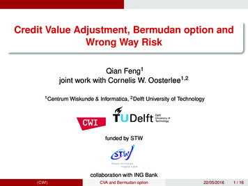
q-forward (Coughlan et al., 2007). For all these securities, the payoff is designed to belinked to the mortality rates of some reference populations at some reference years in thefuture.More recently, Chan et al. (2014) and Tan et al. (2014) proposed a simple longevitylinked security called K-forward to hedge longevity risk. A K-forward is a zero-couponswap that exchanges on the maturity date some fixed amount for a floating amount thatis proportional to a mortality index in the Cairns–Blake–Dowd (CBD) mortality modelfor a certain population. Figure 1 shows the payoffs on the maturity date of a typicalK-forward. The longevity-risk hedger plays the role as the fixed rate receiver and thehedge provider as the fixed rate payer in this contract. If the mortality index turns outto be lower than expected and thus there is a longevity loss, the hedger will get a positive payment from the hedge provider to cover the loss. Compared with other longevityhedging instruments, a big advantage of K-forwards is that their final payoffs only depend on some time-varying mortality index and there is no need to specify a specifichedging age. This feature makes a K-forward longevity hedge easier to implement andthus more conductive to the development of liquidity.Figure 1 is here.Like other longevity-linked securities, K-forward is supposed to be traded over thecounter. Thus, it is necessary to measure its counterparty risk. However, very few papers in the literature have studied counterparty risk in longevity-linked securities untilrecently Biffis et al. (2016) investigated the cost of bilateral default risk and collateral rulesin longevity swaps. In particular, they assumed that the credit risk of the hedge supplieris equal to the average credit quality of the LIBOR panel and thus its default intensityfollows the LIBOR-Treasury spread. In this paper, we propose a framework to evaluatecredit value adjustment (CVA) in K-forwards. One advantage of our work is that we areable to estimate the risk-neutral default intensity for an arbitrary hedge supplier giventhat we can collect enough market information, like corporate bonds, reflecting its creditrisk. For simplicity, we consider a K-forward contract without collateral requirements.Also, since the mortality index data is available once a year, we assume that the evaluation of the K-forward can be done only at the end of each year after the mortality indexdata for that year is available. The CVA at time 0 can be approximated as follows:TCVA (1 R) DF(t) · EE(t) · ( F (t) F (t 1)),(1.1)t 1where 1 R is the loss given default (LGD), which is the percentage of the exposure to belost at default of the counterparty, DF(t) is the risk-free discount factor for time t, EE(t) is2
the expected risk exposure for the institution at time t, and F (t) is the counterparty’s riskneutral default probability by time t. See Gregory (2015; Appendix 14) for the detailedderivation of formula (1.1).We want to point out some important underlying assumptions for the plausibility ofusing formula (1.1) to evaluate the counterparty risk in K-forward. First, the recoveryrate is assumed to be exogenously given and fixed. Second, we consider the possibledefault of the hedge provider only and ignore the possibility that the hedger may alsodefault. This assumption may seem unrealistic at first glance. But if we think of thehedger as a pension fund, whose default is mainly due to unexpected improved mortality rate, we would agree that when the hedger’s default risk is high the risk exposureto the hedge provider is likely to be zero. Last, we assume that there is no wrong-wayor right-way risk, i.e., the credit risk exposure is independent with the hedge provider’sdefault time. This assumption is reasonable since banks usually do not have exposuresto the demographics of a population. Based on these assumptions, we can simply accumulate over time the product of the LGD, the risk exposure and the default probabilityto evaluate the counterparty risk as in formula (1.1).Another important issue we want to address regarding formula (1.1) is that we calculate the expected risk exposure under the real-world measure. Usually, since evaluationof CVA is a pricing application, the expected risk exposure should be calculated underthe risk-neutral measure instead of the real-world measure. However, there is essentially no publicly available pricing information on longevity-linked securities with theonly exception for the longevity bond by the European Investment Bank (EIB) in 2004.While the EIB longevity bond had an issue price of 35 basis points below LIBOR, it wasultimately unsuccessfully issued. The lack of real pricing information makes it impossible to derive reliable risk-neutral mortality indexes. It is also the reason why Biffis etal. (2016) assumed that the death time has the same intensity process under both riskneutral and real-world measures. We further want to point out that, as Cox and Pedersen(2000) explained for catastrophe risks, if a future cash flow depends only on mortality related variables, which are assumed independent of financial risk variables, then the cashflow’s expectation under the risk-neutral measure coincides with that under the realworld measure. Hence, in this paper we derive the CBD mortality indexes under thereal-world measure and use them to calculate the expected risk exposure at each timet, which is consistent with market practice where counterparties would agree on a realworld mortality model.The remaining of the paper is organized as follows. In Section 2, we derive the CBDmortality index data for a reference population and fit it by using a vector time-series3
model. The time-series model is used to predict future mortality indexes for the population. In Section 3, we estimate the risk-neutral default probability by calibrating areduced-form default model on market price of bonds. Then, combining results in Sections 2 and 3, we calculate the CVA in K-forwards for two potential hedge providers inSection 4. Some concluding remarks are given in Section 5.2Model for mortality indexesThe multiperiod-ahead forecasting performance of a stochastic mortality model is essential to its application in longevity risk management. From the work of Cairns et al.(2011) and Dowd et al. (2010), we know that the original CBD mortality model (Cairnset al., 2006) is a relatively simple one among a few that can provide acceptable both exante and ex post forecasts, in particular, for senior ages. Recall that the reparameterizedversion of the original CBD two-factor mortality model assumes that q x,t(1)(2)ln κ t κ t ( x x ),1 q x,t(2.1)where q x,t is the probability that an individual aged x at time t will die by t 1, x is(i )the average of the ages used in the dataset, and κt , i 1, 2, called CBD mortality indexes, are time-varying parameters representing period effects. Assuming deaths follow(1)(2)a binomial distribution one can estimate κt and κt using historical mortality rates.(1)Note that κt represents the level of the logit-transformed mortality curve and a reduc(1)tion in κt(2)means an overall mortality improvement. κtlogit-transformed mortality curve and a positive(2)κtrepresents the slope of themeans that mortality at older agesimproves more slowly than at younger ages.Chan et al. (2014) pointed out a unique feature, the so-called new-data-invariant property, of the CBD mortality indexes. In other words, after new mortality data is available(i )and the CBD model (2.1) is updated accordingly, historical values of κt , i 1, 2, will notchange. This is a very important property based on which Chan et al. (2014) proposedthe concept of K-forward. A K-forward could be considered as a zero coupon swap that(1)(2)exchanges a fixed amount with a floating amount proportional to κ T or κ T for a refer(i )ence population in a future reference year T. Denote by κ̃ T the forward mortality index,which is determined at time 0, and by Y the notional amount. The payoff for the fixedrate receiver on the maturity date can be expressed as (i )(i )Y · κ̃ T κ T ,i {1, 2}.(2.2)4
2.1Mortality dataThe mortality data used in this paper is that for US males aged from 30 to 100. Thereason why we choose the age range 30–100 has two folds. First, we want to exclude theaccident hump at younger ages for which the CBD model does not handle well. Second,(2)the average age is 65, the normal age at which people retire in US. So if κ T is lower(2)than κ̃ T then it would result in extra longevity risk from all retiree groups. HumanMortality Database (2016) has mortality data for US males from 1933 to 2014. Althougha structural change should have occurred during this period, see Li et al. (2011), we stilluse all available mortality data for a baseline case in this paper. The historical values of(1)κt(2)and κtare shown in Figure 2.Figure 2 is here.2.2Vector time-series model(1)(2)In the original CBD model the time variation of κt (κt , κt )T is modeled by a bivariate random walk (Carins et al., 2006). However, a random walk cannot explain eitherserial or cross correlation in the series of κt κt κt 1 , though such correlations aresignificantly observed for almost all populations available. Chan et al. (2014) proposedto apply a vector autoregressive moving-average (VARMA) model on κt and found thebest fitting VARMA model for England and Wales male population from 1950 to 2009.Following Chan et al. (2014), we find in this section the best VARMA model describingthe CBD mortality indexes for US male population from 1933 to 2014.Let us denote d κt d 1 κt d 1 κt 1 , d 1, with 0 κt κt . We say that thevector series d κt follows a VARMA(p, q) process ifpq d κ t Φ0 Φ i d κ t i Θ j e t j e t ,i 1(2.3)j 1where Φ0 is a constant vector, Φi ’s and Θ j ’s are coefficient matrices for i, j 1, Φ p 6 0,Θq 6 0, and et is a sequence of independent and identically distributed random vectorswith mean zero and positive-definite covariance matrix Σ. It is known that for a VMA(q)process its cross-correlation matrices with lag q are all zero and for a VAR(p) processits partial autoregressive matrices with lag p are all zero. In addition, assuming thatthe lag-l partial autoregressive matrix is zero, the likelihood ratio statistic M(l ) is asymptotically chi-squared distributed with four degrees of freedom. See Tiao and Box (1981)and Tsay (2014) for more details on properties of VARMA models.For model identification, we employ the sample cross-correlation matrices (SCCM)and the likelihood ratio statistic M(l ) for the sample partial autoregressive matrices to5
help choose the appropriate orders p and q. Table 1 shows SCCM and the likelihoodratio statistic M(l ) for the series κt . Since all SCCM of κt up to lag 8 are significantlynot zero, we turn to the first-order difference κt . Table 2 shows SCCM and M(l ) for κt . Now only the lag-1 and lag-3 SCCM matrices are significantly not zero. We settlewith the first-order difference. Since the critical value for M (l ) is χ24,0.95 9.45, we seethat M (l ) is significantly not zero at lags 1, 3 and 5 only. Based on these observations,we focus on VARMA(p, q) models with p 5 and q 3. Table 3 shows the AkaikeInformation Criterion (AIC) for different fitted VARMA models on κt . VARMA(5, 0)gives the lowest AIC which indicates that (5, 0) could be the best fitted model. Theestimated coefficients and their corresponding standard errors of a VARMA(5, 0) modelfitted on κt are given in Table 4.Tables 1–4 are here.We then do diagnostic checking for the fitted VARMA(5, 0) model. Table 5 showsthe SCCM and M(l ) of the residuals after fitting a VARMA(5, 0) model on κt . SCCMmatrices are insignificant from zero at all lags and M (l ) are all less than the critical valueχ24,0.95 9.45. We further check the normality assumption on errors since we are goingto assume normality in simulation later. Table 6 shows the p-value and conclusion ofnormality tests on the residuals after fitting a VARMA(5, 0) model on κt . The residualspass all the following three multivariate normality tests at 5% significance level: Royston’s test, Henze–Zirkler’s test, and Mardia’s test.Tables 5–6 are here.In the end we want to point out that our choice of the VARMA(5, 0) model for κtis consistent with the one chosen by Chan et al. (2014), who studied the CBD mortalityindexes for England and Wales male population from 1950 to 2009.2.3BacktestingThe ex post forecasting performance of the fitted mortality model is important since reliable evaluation of CVA in K-forward would heavily depend on acceptable predictions offuture mortality indexes that do not differ significantly from realized outcomes. Dowdet al. (2010) proposed a backtesting framework and applied it on a variety of stochasticmortality models. In particular, they investigated the out-of-sample predicting performance of the CBD mortality model by assuming that κt follows a bivariate random walkwith drift. In the remaining of this section, we will perform similar backtesting underthe assumption that κt follows a VARMA process.6
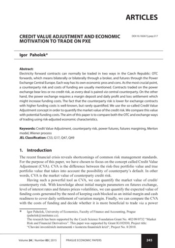
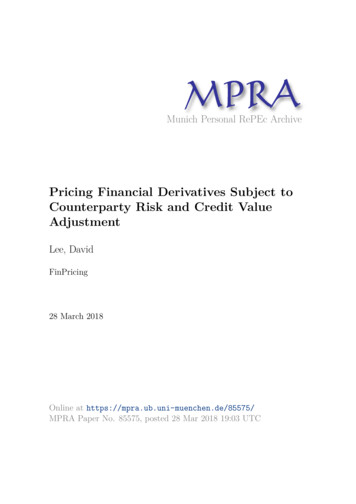
According to Tsay (2014, Chapter 3), if a VARMA process (2.3) holds with d 1, then κt has a moving-average representation κt µ Ψi et i ,i 0where µ (I Φ1 ) 1 Φ0 , Ψ0 I, Ψ1 Φ1 Θ1 , Ψi Φ1 Ψi 1 , i 2, 3, . . ., and I is the2 2 identity matrix. So we are able to derivett t ii 1i 1 j 0κt κ0 κi κ0 tµ Ψ j ei i t Ψ j e i .i 0 j i 1Suppose that we are at time 0 and try to predict t steps ahead. Denote κ(t) E(κt F0 )with F0 being the available information at time 0. Then,t t i Ψ j eiκt κ(t) i 1 j 0andcov (κt κ(t)) tt ii 1j 0 Ψj!·Σ·t i ΨTj!.j 0(1)Figure 3 shows the 95% prediction interval and median prediction line of κt(2)κtandfrom 2000 to 2014 based on the mortality index data up to 1999. If the fitted modelis proper, we would expect no more than 5% real mortality index turn out to fall outside(1)of the confidence interval. It is clear that all real outcomes κt from 2000 to 2014 fall(2)within the interval. As for κt , only one out of fifteen real outcomes exceeds the intervalboundary. Given that we have a relatively short forecast horizon (15 years), the ex post(1)forecasting performance on both κt(2)and κtis acceptable.Figure 3 is here.We also perform another backtest based on a formal statistical hypothesis test. Againwe use the CBD mortality index data from 1933 to 1999. After fitting a VARMA(5,0)model on κt , we can forecast by simulation the cumulative distribution function for(1)(2)κt and κt in future years. The null hypothesis is that the realized mortality indexesare consistent with their predicted distribution functions. Then by locating the realized(i )κt , i 1, 2, on its predicted distribution function curve, we can obtain its p-value, whichis associated with the left-sided test of the null hypothesis. Note that here we focus onleft-sided tests since if the model cannot generate adequate outcomes smaller than the(i )realized κt , i 1, 2, then it is not reliable to hedge longevity risk. The results are shown7
(1)in Figure 4. It can be clearly seen that the model does a good job in predicting κt . Its(2)p-values at all 15 horizon years are all greater than 10%. The p-value for κtdrops below(1)5% significance level only for the last two years in the forecast horizon. Given that κt(i )carries the main part of the longevity risk, as can be seen from the variations of κt ,i 1, 2, in Figure 2, the model has an acceptable performance in this backtest as well.Figure 4 is here.3Risk-neutral default probabilityIn this section we employ a parametric reduced-form model to describe the default behaviour of a hedge provider. Given a set of non-callable bonds issued by the hedgeprovider, we try to match their “dirty prices” implied from the reduced-form model withtheir market prices. In this way we are able to determine the optimal set of parametersthat gives us the best estimate for the hedge provider’s risk-neutral default probabilitywithin a finite time horizon.We assume that at time 0 the forward default intensity of the hedge provider is adeterministic positive function of time t, which has the formh(t; β) β 0 β 1 e t/β3 β 2 e t/β3 t/β 3 ,t 0,(3.1)with β ( β 0 , β 1 , β 2 , β 3 )T R4 . If β satisfies that h(t; β) 0 for all t 0, then it isstraightforward to derive the cumulative hazard rate function and the survival probability as1H (t; β) tZ t0h(s; β)ds β 0 ( β 1 β 2 )(1 e t/β3 ) β 3 /t β 2 e t/β3(3.2)andS(t; β) exp ( tH (t; β)) ,t 0.(3.3)The function h(t; β) in (3.1) was first proposed by Nelson and Siegel (1987) to modela bond’s yield curve. Duan et al. (2012) also found it useful in smoothing parameterswhen modeling forward default intensity. A great advantage of this parsimonious modelis that all of the parameters have their own economic meanings. Indeed, β 0 is the longterm converging value of the default intensity, β 1 and β 2 represent the short-term andmedium-term effects for the default intensity, respectively, and β 3 0 acts as the timescalar parameter. In our application, since the default intensity is always positive, werequire S(t; β) in (3.3) to be a decreasing survival function, which means that, given β,8
S(0; β) 1, limt S(t; β) 0, and S0 (t; β) 0 for all t 0. Thus, besides β 3 0 weneed the following additional constraints on β:(C1) β 0 0;(C2) β 0 β 1 0;(C3) β 2 β l with β l uniquely satisfying β l β 1 and β 0 β l exp ( β 1 /β l 1) 0.See Appendix A for the proof of the fact that constraints C1–C3 together is equivalent tothat S(t; β) is a decreasing survival function.3.1Model calibrationFor a potential hedge provider, we estimate its risk-neutral forward default intensityby calibrating model (3.1) according to its available bond prices. Specifically, supposewe have detailed information, including market price, coupon rate, principal, maturity,etc., of K non-callable bonds issued by the hedge provider. The bond information iscollected on the same day, which is considered as time 0. By combining discountedfuture coupon/principal payments with survival probability from (3.3), we are able tocalculate the so-called “dirty price” for each bond asnZ snj 10 DF(s j ) · c j · S(s j ) V · DF(sn ) · S(sn ) V · R ·DF(s) F (ds).(3.4)In the above formula, s j , j 1, . . . , n, are the coupon payment moments with sn thematurity, c is the coupon rate, j is the fraction of years between s j 1 and s j , V is thepar value, R is the recovery rate, DF(·) is the risk-free discount factor, S(·) S(·; β) forsimplicity, and F (·) 1 S(·). Note that in order to derive formula (3.4) we assume thatthe recovery is a fraction of the par value. Next we perform a calibration process on β,under constraints C1–C3, such that the mean absolute error is minimized as1β arg minKβ K dirty pricek market pricek .(3.5)k 1By doing so, we find for the hedge provider the optimal set of parameters β that bestmatches each bond’s market price with its dirty price. Then we are able to use h(t; β ) asthe proxy for the hedge provider’s risk-neutral forward default intensity.We perform the model calibration process for two potential hedge providers: JP Morgan (JPM) and Royal Bank of Scotland (RBS), who have participated in transactionsof longevity-linked securities in the last decade. See, for example, Table 1 of Biffis etal. (2016). The bond information of JPM and RBS, all retrieved on June 16, 2016 fromBloomberg database, is summarized in Tables 7–8, respectively.9
Tables 7–8 are here.Since all bonds are in US dollars, we use US Treasury zero yields on the same day tocalculate the risk-free discount factor. Note that almost all of the bonds are senior unsecured except that two of RBS are subordinated. According to Table 24.2 of Hull (2014),the average recovery rate, as a percentage of par value, of senior unsecured corporatebonds in the period 1982–2012 is about 37%. Hence, we assume the fixed recovery rateR 37% in the dirty price formula (3.4). We also want to point out that the optimizationin (3.5) is nonlinear with multiple constraints, which is not trivial. We implement it in R3.3.1 (R Core Team, 2016) using the NLopt package (Johnson, 2008).The comparison of bonds’ market prices and their dirty prices after model calibrationis demonstrated in Figures 5–6. It is clear that the overall matching performance is verygood with a mean absolute error of 0.496 dollars for JPM’s ten bonds and of 0.923 dollarsfor RBS’s seven bonds. Among all seventeen bonds, sixteen bonds have a percentagediscrepancy less than 1.5% between dirty price and market price while there is only oneexception at 4.5%.Figures 5–6 are here.We also look at the estimated risk-neutral credit spread term structure of the two banks.Here the credit spread at time t is simply defined as (1 R) H (t; β). The left plot in Figure 7 displays JPM’s credit spread term structure estimated by assuming β βJPM(0.0125, 0.0050, 0.0181, 2.8895)T . The credit spread curve is hump shaped, increasing upto around 5 years and then keeping decreasing beyond that point. This is a genericB-rating credit spread curve according to Lando and Mortensen (2005). Similarly, theright plot in Figure 7 displays RBS’s credit spread term structure estimated by assuming β βRBS (0.0210, 0.0170, 0.0676, 4.9448)T . Again, the credit spread curve is humpshaped with the peak at around the 5-year point. But compared with that of JPM, thecredit spread curve of RBS clearly shifts to a much higher level.Figure 7 is here.So we find something interesting here. According to Moody’s, JPM’s senior unsecuredbonds are rated at A3 in the category of medium grade and RBS’s senior unsecured bondsare rated at Ba1 in the category of non-investment grade speculative. However, their riskneutral credit spread curves, estimated based on their public-traded bonds, both behavelike a B-rating one, which belongs to the highly speculative category. This indicates thatthe financial market is very risk averse when pricing credit risk.10
4CVA of K-forwardIn this section we calculate CVA of K-forwards for a pension fund. We assume thatthe pension fund and a hedge provider have an agreement of K-forwards written onUS male population as described in Section 2. The two potential hedge providers weconsider in this paper are JPM and RBS. We use the CVA evaluation formula (1.1), inwhich the risk exposures are calculated by applying the vector time-series model onthe CBD mortality indexes κt as in Section 2 and the risk-neutral default probability isestimated by calibrating the reduced-form model on the hedge provider’s bond pricesas in Section 3. Next we state the assumptions and steps of our calculation before wepresent the numerical results in Section 4.1.We assume time 0 as on June 16, 2016, on which date we collected bonds’ informationfor the two potential hedge providers. The K-forwards are used to hedge longevity riskfor up to 25 years beyond 2016. Denote by κ0 the mortality indexes of year 2016, by κ1 themortality indexes of year 2017, and so on. In practice, there is usually a time lag betweenthe end of a reference year and the availability of the mortality index data for that year.For simplicity, we suppose in this paper that κt for each year starting 2016 are availableon December 31 of the same year. At the end of each year t we can obtain an updatedestimate of κ T by applying the fitted VARMA model to the realization of κt up to yeart. We then plug the updated estimates of κ T in formula (2.2) to get the risk exposures ofthe K-forwards at year t. The CVA is an accumulation up to year T of the discounted riskexposure combined with the default probability and the loss given default. The detailedsimulation procedure is as follows:Step 1: Simulate a sample path of κt , t 0, 1, . . . , T, based on the historical mortalityindexes κt and the fitted VARMA(5, 0) model on κt .Step 2: At the end of each year t 0, 1, . . . , T, update the estimate of κ T based on thesimulations up to year t from Step 1. Compare it with the original value estimatedat time 0 to determine the risk exposure at that point.Step 3: For each risk exposure at the end of year t in Step 2, multiply it with the marginalrisk-neutral default probability in year t, the risk-free discount factor correspondingto the end of year t, and the loss given default.Step 4: A realization of CVA is obtained by adding together all the products for yearst 0, 1, . . . , T, in Step 3.Step 5: Repeat Steps 1–4 for 1,000,000 times. The average CVA is our final estimate.11
4.1Numerical resultsThe numerical results of CVA measured in basis points (bpts) for K1-forward and K2forward are summarized in Table 9.Table 9 is here.Our first observation is that for US male population the CVA of K1-forward is alwaysmuch larger than that of K2-forward. For instance, the CVA of K1-forward at T 25years is 52.4 bpts for JPM, more than half of the corresponding credit spread (95.4 bpts),while the CVA of K2-forward for the same reference year is only 1.6 bpts, which is almost(1)negligible. The big discrepancy in CVA values is actually due to the fact that κt mea(2)sures the level of the whole logit-transformed mortality curve while κtrepresents theslope of the logit-transformed mortality curve. In Figure 2 we can easily see that for US(1)male population the fluctuation in κt contains the main part of the longevity risk andbears a larger uncertainty along with time. It would be interesting to know if this relationship between K1-forward and K2-forward holds for other populations as well giventhat some populations, like Canadian male as found by Chan et al. (2014), may have(1)(2)relatively less uncertainty associated with κt but more uncertainty associated with κt .Second, the CVA of K-forward is greatly influenced by the hedge provider’s creditrating. As we introduced in Section 3, the long-term credit rating of JPM is A3, whichbelongs to the category of medium grade, while that of RBS is Ba1, which is in the category of non-investment grade speculative. As a result, the credit spreads of RBS at years15, 20 and 25 are all as about two and a half times as that of JPM. Similarly, for both K1forward and K2-forward, CVA of RBS is almost as double as that of JPM. The differentlevels of scaling confirm that CVA, unlike credit spread which is the risk premium for aspecific time point, depends essentially on the whole credit curve of the hedge provider.This also makes it very important to accurately estimate the whole credit curve, not onlycredit spreads at some time points, in order to obtain a reliable estimate of CVA.Last we want to talk about the impact of recovery rate. We fix the recovery rate at 37%in the above calculation only because it is the historically average recovery rate of seniorunsecured corporate bonds. But in reality the recovery rate is not known at issuanceand its realized value could be any number between 0 and 1. We calculate the CVAsagain by assuming that financial market believes the hedge provider might default witha recovery rate of 25% and 50%, respectively. The results are summarized in Tables 10–11.It can be clearly seen that the randomness of recovery rate has a big impact on CVA fora hedge provider with non-investment grade, like RBS. For instance, when the assumedrecovery rate drops from 50% to 37%, corresponding to a 26% increase of LGD, the CVA12
of K1-forward at year 25 for RBS increases by 33.8%!Tables 10–11 are here.5Concluding remarksIn this paper, we propose a baseline framework to calculate CVA in K-forward. Therisk exposure part is obtained by applying a VARMA model on mortality indexes. Therisk-neutral default probability is derived from a red
Evaluation of Credit Value Adjustment in K-forward Xuemiao Hao, Chunli Liangy, Linghua Wei z April 27, 2017 Abstract We model and quantify counterparty credit risk for K-forward, a newly proposed longevity-linked security. We focus on the evaluation of credit value adjustment (CVA) from the longevity risk hedger's perspective. The modeling .