Transcription
Computing Credit Valuation Adjustment solvingcoupled PIDEs in the Bates modelLudovic Goudenège, Andrea Molent, Antonino ZanetteTo cite this version:Ludovic Goudenège, Andrea Molent, Antonino Zanette. Computing Credit Valuation Adjustmentsolving coupled PIDEs in the Bates model. Computational Management Science, Springer Verlag,2020, 17 (2), 10.1007/s10287-020-00365-6 . hal-01873346 HAL Id: 1873346Submitted on 14 Sep 2018HAL is a multi-disciplinary open accessarchive for the deposit and dissemination of scientific research documents, whether they are published or not. The documents may come fromteaching and research institutions in France orabroad, or from public or private research centers.L’archive ouverte pluridisciplinaire HAL, estdestinée au dépôt et à la diffusion de documentsscientifiques de niveau recherche, publiés ou non,émanant des établissements d’enseignement et derecherche français ou étrangers, des laboratoirespublics ou privés.
Computing Credit Valuation Adjustment solving coupled PIDEsin the Bates modelLudovic Goudenège Andrea Molent†Antonino Zanette‡AbstractCredit value adjustment (CVA) is the charge applied by financial institutions to the counterparty tocover the risk of losses on a counterpart default event. In this paper we estimate such a premium under theBates stochastic model (Bates [4]), which considers an underlying affected by both stochastic volatility andrandom jumps. We propose an efficient method which improves the finite-difference Monte Carlo (FDMC)approach introduced by de Graaf et al. [11]. In particular, the method we propose consists in replacing theMonte Carlo step of the FDMC approach with a finite difference step and the whole method relies on theefficient solution of two coupled partial integro-differential equations (PIDE) which is done by employing theHybrid Tree-Finite Difference method developed by Briani et al. [6, 7, 8]. Moreover, the direct applicationof the hybrid techniques in the original FDMC approach is also considered for comparison purposes. Severalnumerical tests prove the effectiveness and the reliability of the proposed approach when both European andAmerican options are considered.Keywords : Credit Value Adjustment, Hybrid methods, PIDE, Monte Carlo, Bates model. Féderationde Mathématiques de CentraleSupélec - CNRS FR3487, France - ludovic.goudenege@math.cnrs.frdegli Studi di Udine, Italy - andrea.molent@uniud.it‡ Dipartimento di Scienze Economiche e Statistiche, Università degli Studi di Udine, Italy - antonino.zanette@uniud.it† Università1
1IntroductionFinancial institutions suffer several risks, one of them is the counterparty credit risk (CCR). This risk arisesfrom the possibility that the counterparty of a financial contract may default. This risk was often overlooked,but in the last decades, after the financial crisis of 2007 and the Lehman Brothers failure in 2008, it gainedmore and more interest by practitioners and academics. In particular, according to the Basel III frameworkof 2010, financial institutions must charge a premium to their counterparty according to its credit reliabilityin order to compensate for a possible counterparty default. Also IFRS 13 in 2013 requires the fair value offinancial products to be measured based on counterparty credit risk. For these reasons, financial institutionscharge to the counterparty a premium called Credit Valuation Adjustment (CVA), which is the differencebetween the risky value and the current risk-free value of derivatives contract. Estimating the good value ofthe CVA can be a demanding effort due to its complicated definition and to its dependence by the underlyingstochastic model. As no specific method is prescribed in the accounting literature, various approaches areused in practice by derivatives dealers and by end users to estimate the effect of credit risk on the fairvalue of financial derivatives. The common approach is to price the CVA through the so called expectedexposure, which is the mean exposure distribution at a future date. Usually, this exposure is calculated bymeans of Monte Carlo approaches which are computationally expensive. In particular, nested Monte Carlosimulations or least squares techniques are employed by Joshi and Kwon [20]. These techniques have beenimproved through the use of stochastic grid bundling method by Jain and Oosterlee [19] and by Karlson etal. [21]. An interesting approach to compute the CVA - when the Heston model is assumed - is the so calledfinite-difference Monte Carlo (FDMC) method, proposed by de Graaf et al. [11]. Such an approach combinesthe finite-difference method and the Monte Carlo method to solve a partial differential equation (PDE) andto estimate the mean exposure respectively. Feng [12] adapted the FDMC approach to deal with the caseof an underlying evolving according to the Bates model: in this particular case, the PDE to be solved isreplaced by a partial integral differential equation (PIDE), which implies an additional computational effort.Other recently introduced alternative approaches consist in employing the fast Fourier transform (Borovykhet al. [5]) or marked branching diffusions (Henry-Labordère [17]).In this paper we focus on the computation of the CVA when the Bates model is considered and we proposean efficient method which improves the results of the FDMC method. Specifically, the Bates model considersan underlying affected by both stochastic volatility and random jumps: the dynamics of the underlying assetprice is driven by both a Heston stochastic volatility [18] and a compound Poisson jump process of the typeoriginally introduced by Merton [22]. Such a model was introduced by Bates [4] in the foreign exchangeoption market in order to tackle the well-known phenomenon of the volatility smile behavior. In the caseof plain vanilla European options, Fourier inversion methods, employed by Carr and Madan [9], lead toclosed-form formulas to compute the price under the Bates model. Two innovative and efficient approachesto price derivatives when the Bates model is considered are proposed by Briani et al. [6], the so called HybridTree-Finite Difference method and Hybrid MC method.Our main result consists in developing an efficient numerical method to estimate the CVA. In particular,the method we propose consists in computing the CVA value as the solution of two coupled PIDE – one forthe risk free price and one for the risk adjusted price – which are solved by means of the Hybrid Tree-FiniteDifference method. That is, we replace the Monte Carlo step in the FDMC method with the computationof the solution of a PIDE and this improves clearly the computational efficiency.Moreover, the direct application of the hybrid techniques in the original FDMC approach is considered forcomparison purposes. Specifically, we apply the two hybrid methods developed by Briani et al. to performboth the finite difference step and the Monte Carlo step of the FDMC approach.Several numerical experiments show that the proposed method is efficient and reliable as it providesaccurate approximations for the CVA value with a low computational cost.The reminder of the paper is organized as follows. Section 2 introduces the Bates stochastic model andthe partial integro-differential equation that allows one to compute option prices. Section 3 presents theCVA definition and some useful properties used in the following. Section 4 outlines the main features of thehybrid methods and how to employ them in option pricing. Section 5 describes the numerical methods forcomputing the CVA. Section 6 presents and discusses the results of the numerical simulations. Section 72
concludes.2The ModelIn the Bates model the volatility is assumed to follow the CIR process (Cox et al. [10]) while the underlyingasset price process contains a further noise from a jump process. In particular, the model for the stock priceand its volatility is given by the following relations:pdSt (r η)dt Vt dZtS dHt ,St (2.1) dVt κ(θ Vt )dt σ Vt dZtV ,where η denotes the continuous dividend rate, S0 , V0 are positive values, Z S , Z V are correlated Brownianmotions such that dZts , dZtV ρdt and H is a compound Poisson process with intensity λ and i.i.d. jumps{Jk }k , that isKtXHt Jk ,(2.2)k 1K denoting a Poisson process with intensity λ. As in the model of Merton [22], we assume that the jumpsare i.i.d. log-normal random variables, described by β2 2(2.3),β ,log (1 J) N α 2with α and β real parameters.We consider an option with maturity T 0, payoff function ψ (S) and we denote with V (t, S, V ) its fairprice at time t, if St S and Vt V . Then, the price of the derivative V is then given byhiV (t, S, V ) E e r(T t) ψ (ST ) S0 S, V0 V .(2.4)Using a martingale approach for an European option, it is possible to show that V (t, S, V ) satisfies thefollowing partial integro-differential Equation (PIDE) (Salmi et al [25]): 2 V (t, S, V ) 1 2 2 V (t, S, V ) V (t, S, V ) 2 V (t, S, V ) V (t, S, V ) 1 ρσVS (r q λ (eγ 1)) V S2 σ V t2 S 2 S V2 V 2Z S V (t, S, V ) κ (θ V ) (r λ) V (t, S, V ) λV (t, xS, V ) pJ (x) dx 0, (2.5) V0with the terminal condition isV (T, S, V ) ψ (S) ,(2.6)where pJ (x) is the log-normal probability density function of the jump variable J.We define the following operators: 2V V 2V1 2V V1 (r q λ (eγ 1)) σ2 V κ (θ V ) (r λ) V,LC V V S 2 2 ρσV S22 S S V2 V S V(2.7)andLJ V λZ0 V (t, xS, V ) pJ (x) dx.(2.8)Therefore, by using (2.7) and (2.8), the PIDE (2.5) can be rewritten in the more compact form as follows: V (t, S, V ) LC V (t, S, V ) LJ V (t, S, V ) 0. t3(2.9)
3The CVALet us define the exposure (or financial exposure) E (t) towards a counterparty at time t as the positive sideof a contract (or portfolio) value V (t, St , Vt ), that isE (t) max [V (t, St , Vt ) , 0] .(3.1)This amount represents the maximum loss if the counterparty defaults at t: an economic loss would occurif the transactions with the counterparty has a positive economic value at the time of default (see the BaselCommittee [3]).Let us define the present Expected Exposure (EE) at a future time t T asEE (t) E [E (t) F0 ](3.2)where F0 is the filtration at time t 0. In particular, in the case of a long position in a Call or Put option,the price is always positive and thus the EE is equal to the future option price.Let τC denote the counterparty’s default time: such a time is a random variable which is supposed to beindependent from the stochastic processes Z S , Z V and H. Moreover, we describe its cumulative distributionfunction as follows: Z t P D (t) 1 exp δ (s) ds .(3.3)0R Here, δ (t), the so called hazard rate, is a non-negative function such that 0 δ (s) ds (Promislow[23]). If the counterparty has not defaulted yet, then δ (t) dt is the probability that it would default betweent and t dt. The possibility of counterparty default reduces the value of the option as in case of default theholder does not receive the whole value of the option. In particular, the holder can recover only a percentageof the contract value, which is called the recovery rate R. The CVA is defined as the difference between therisk free price and the risk adjusted price. More precisely, as stated by Gregory [15], the CVA is given by:Z TCVA (1 R)D (0, s) EE (s) dP D (s) ,(3.4)0where D (0, t) is the risk-free discount factor. This mean that the CVA is the expected value of the possiblelosses due to counterparty default. We stress out that definition requires the exposure and the counterpartiesdefault probability to be independent and the discount factor to be also independent of the exposure. Usingequations (3.2) and (3.4), we obtain the following relation:#"ZT(3.5)CVA ED (0, s) (1 R) E (s) dP D (s) F0 .0According to (3.5), the CVA is the price (mean value of the future cash flows) of a financial derivative whichpays (1 R) max [V (τC , SτC , VτC ) , 0] at time τC . Therefore, we can consider the CVA as a derivative itselfand we denote its financial value at time t with C (t, St , Vt ), that is"Z#TC (t, St , Vt ) ED (0, s) (1 R) E (s) dP Ds Ft ,thaving CV A C (0, S0 , V0 ). It is possible to show that C (t, St , Vt ) solves the following PIDE (see theAppendix for more details): P D C (t, S, V ) LC C (t, S, V ) LJ C (t, S, V ) (1 R) max [V (t, St , Vt ) , 0](t) 0, t twith the terminal conditionC (T, S, V ) 0.(3.6)(3.7)We stress out that equation (3.6) depends on the value V (t, St , Vt ) which has to be computed previouslyby solving equation (2.9).4
4Hybrid methods in the Bates modelThe Hybrid Tree Finite Difference (HTFD) and the Hybrid Tree Monte Carlo (HTMC) methods are twoinnovative and efficient approaches to price derivatives when the Bates model is considered. In this Sectionwe present the main ideas that underlie these two methods: the interested reader can find more details aboutthe numerical procedures in Briani et al. [6].4.1The HTFD methodThe HTFD method is a backward induction algorithm that works following a finite difference PIDE methodin the direction of the share process and following a tree method in the direction of the other randomsources, that is volatility in the case of Bates model. Specifically, the method is based on the following steps.First of all, a binomial tree for the CIR volatility process V is considered according to Apolloni et al. [2].Then, a transformation which keeps the diffusion processes S and V uncorrelated is applied. Finally, a finitedifference approach in the S-direction is developed.In particular, consider a large integer value N , a time horizon [0, T ] and define h T /N . For n 0, 1, . . . , N , defineVnh {vn,k }k 0,1,.,n(4.1)withvn,k We define the multiple jumps p 2σV0 (2k n) h 1 V0 σ (2k n) h 0 .22(4.2)kdh (n, k) max {k : 0 k j and vn,k µV (vn,k ) h vn 1,k } ,kuh (n, k) min {k : k 1 k n 1 and vn,k µV (vn,k ) h vn 1,k }in which µV denotes the drift coefficient of V , that is µV (v) κ (θ v). Starting from the node (n, k),the discrete process can reach the up-node n 1, kuh (n, k) or the down-jump node n 1, kdh (n, k) withtransition probability given byup-jump: phkh (n,k) 0 uµV (vn,k ) h vn,k vn 1,kdh (n,k)vn 1,kuh (n,k) vn 1,kdh (n,k)down-jump : phkh (n,k) 1 phkuh (n,k) .d 1,(4.3)(4.4)Multiple jumps and jump probabilities are set in order to match the first local moment of the tree and of theprocess V up to order one with respect to h. As a consequence, as h approaches to 0, the weak convergence onthe path space is guaranteed. Moreover, in order to obtain the convergence, the Feller condition (Albrecheret al. [1]) is not required.Let us consider the diffusion pair (Y, V ), where Y is a stochastic process defined byYt log (St ) ρVt .σ(4.5)pClearly the couple (S, V ) can be retraced by (Y, V ) by inverting relation (4.5). We set ρ̄ 1 ρ2 and weconsider (W, Z) as a standard Brownian motion in R2 . Then, the dynamics of the couple (Y, V ) is given by pρ1dYt r η Vt κ (θ Vt ) dt ρ̄ Vt dZt dNt ,(4.6)2σpdVt κ (θ Vt ) dt σ Vt dWt ,(4.7)5
with Y0 log S0 σρ V0 . Here, Nt is the compound Poisson process written through the Poisson process K,with intensity λ, and the i.i.d. jumps {log (1 Jk )}, that isNt KtX(4.8)log (1 Jk ) .k 1We setρ1µY (v) r η v κ (θ v)2σ(4.9)µV (v) κ (θ v) .(4.10)andLet V̄ h V̄n hn 0,.,Nhdenote the tree process approximating V and set Vth V̄⌊t/h⌋, t [0, T ], theassociated piecewise constant and cà dlà g approximation path. In order to approximate Y , Briani et al.construct a Markov chain from the finite difference method. Starting from the Euler scheme Y0h Y0 andfor t (nh, (n 1) h], n 0, . . . , N , it is possible to setq hhh (Z Z ) (N N ) ,(t nh) ρ̄ Vnh(4.11)Yth Ynh µY Vnhtnhtnh Z being independent of the noise driving V̄ h . Now, let W (t, Y, V ) V t, exp Y σρ V , V the functionwhich gives the price of the financial derivative at time t in terms of the couple (Y, V ) . Then, hhE W (n 1) h, Y(n 1)h , V(n 1)h Ynh y, Vnh v E W (n 1) h, Y(n 1)h, V(n 1)h Ynh y, Vnh v(4.12) hh Vnh v E uh nh, y; v, V(n 1)hwhereand (4.13) hhhuh (nh, y; v, z) E W (n 1) h, Y(n 1)h, z Ynh y, Vnh v(4.14)uh (nh, y; v, z) uh (s, y; v, z) s nh .(4.15)The key point of the HTFD method is that the function (s, y) 7 u (s, y; v, z) solves the following PIDE inthe time interval nh s (n 1) h:Z h uh 1 2 2 uh uhu (s, y x; v, z) uh (s, y; v, z) pJ (x) dx 0,(4.16) µY (v) ρ̄ v2 s y2 y hfor y R, and with terminal condition given byuh ((n 1) h, y; v, z) W ((n 1) h, y, v) .(4.17)In order to numerically solve the PIDE (4.16) by using a finite difference scheme, we first localize thevariables and the integral term to bound the computational domains. For this purpose, we use the estimatesfor the localization domain and the truncation of large jumps given by Voltchkova and Tankov [26]. Then,the derivatives of the solution are replaced by finite differences and the integral terms are approximatedusing the trapezoidal rule. Finally, the problem is solved by using an explicit-implicit scheme.We observe that the above algorithm is referred to a European option, can easily be adapted to consideran American option. Specifically, we approximate the American option with a Bermudan option with exercisedates given by the set {nh}n 0,.,N and replacing equation (4.17) with the following one:h ρ iuh ((n 1) h, y; v, z) max W ((n 1) h, y, v) , ψ exp y v(4.18)σWe stress out that the computation of uh as the solution of (4.16) is a one dimensional problem withconstant coefficients, thus it can be solved in a very efficient way, with a low computational cost.6
4.2The HTMC methodThe HTMC method is a Monte Carlo algorithm which is based on the approximations (4.3) and (4.11).In particular, the HTMC method consists in simulating a continuous process in space (the component Y )starting from a discrete process in space (the 1-dimensional tree for V ). In particular, we set Ŷ0h Y0 forht [nh, (n 1) h] with n 0, 1, . . . , N 1. Then, we compute Ŷn 1recursively by the following relation:hŶn 1 Ŷnhq h µY V̂n h ρ̂ hV̂nh n 1 N(n 1)h Nnh(4.19)where 1 , . . . , N are i.i.d. standard normalrandom variables which are independent of the noise driving the Markov chain V̂ and N(n 1)h Nnh is the compound Poisson increment. Roughly speaking, one letthe pair (Y, V ) evolve on the tree and simulate the process Y at time nh by using relation (4.19).5Numerical method for computing the CVAIn this section we present the proposed approach to compute the CVA, namely the Coupled-Hybrid TreeFinite Differences (C-HTFD), which is based on the resolution of two coupled PIDE. Moreover, we startpresenting the Hybrid Tree Finite Difference-Hybrid Monte Carlo (HTFD-HTMC) method which is based onthe direct application of the hybrid techniques in the original FDMC (we consider this method for comparisonpurposes mainly). The two approaches are both based on the application of the hybrid algorithms of Brianiet al. [6], presented in Section 4.5.1The HTFD-HTMC approachThis method is based on the direct application of the hybrid techniques to the Finite Difference MonteCarlo (FDMC) method, which was first developed by de Graaf et al. [11] for the Heston model and thenadapted for the Bates model by Feng [12]. First of all, an estimation of the value function V (t, S, V ) iscomputed through a grid of values by solving equation (2.5) by employing the Alternating Direction Implicit(ADI) method and specifically the scheme proposed by Haentjens and In’t Hout [16]. Then a Monte Carlosimulation is employed to estimate the expectation in (3.4) and thus estimate the CVA.In the HTFD-HTMC approach we employ the HTFD method to solve (2.5) and the HTMC method to estimate (3.4). Specifically, let h T /N as in Subsection 4.1. First of all, the HTFD method is used to computethe risk free price {V (nh, Snh , Vnh )}n 0,.,N at discrete times {0, h, . . . , N h}. Then, we estimate the expectedon jjexposure (3.2) via a set of NMC Monte Carlo simulationsSnh, Vnh, n 0, . . . , N and j 1, . . . , NMCgenerated via the HTMC method, that isEE (nh) 1NMCNMCXj 1h ijjmax V nh, Snh, Vnh.(5.1)Finally, we compute the CVA by approximating the integral in (3.4) using the uniform partition {0, h, . . . , N h}of [0, T ], the estimated value {EE (nh) , n 0, . . . , N } and the trapezoidal rule.5.2The C-HTFD approachFirst of all, an estimation of the value function V (t, S, V ) is computed through a grid of values by solvingequation (2.5) by means of the HTFD method. Then, the CVA is computed as the solution of the PIDE(3.6), which is done again by employing the HTFD method. We stress that C-HTFD method and theHTFD-HTMC method share the first step, but in the C-HTFD method the Monte Carlo step is replacedwith a second finite difference like step.7
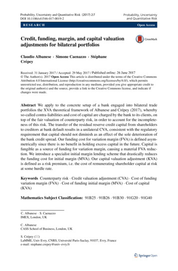
6Numerical ResultsIn this section we propose the results of some numerical experiments, which aim to compare the goodnessof the proposed methods. In particular, we compare the standard FDMC method employed by Feng [12],the HTFD-HTMC approach and the C-HTFD approach. We employ the numerical methods according to4 configurations (A, B, C, D), each of them with an increasing number of steps, determined in order toachieve approximately these run times1 : (A) 0.25 s, (B) 1 s, (C) 4 s, (D) 16 s. The employed mesh andconfiguration parameters are reported in Table 1. Specifically, for the FDMC method with the sequence(time steps - points for S - points for V - MC simulations) and for the hybrid methods with the sequence(time steps - points for Y - MC simulations). Moreover, we reported the 95% confidence intervals for theFDMC method and for the HTFD-HTMC.Furthermore, we employ the FDMC method with a huge number of steps and paths 250; 500; 200; 106 as a benchmark (BM ).We consider the following parameters for the Bates model: S0 80, 100, 120, K 100 , T 1, r 0.03,η 0.00, V0 0.01 κ 2, θ 0.01, σ 0.2, λ 0.1, α 0.1, β 2 0.1 and ρ 0.5. According to thedefault parameters, we consider δ (t) δ 0.03 and R 0.4. We compute the CVA for a European and anAmerican a Put option with strike equal to K 100.Results are available in Tables 2 and 3, which show that all the implemented methods give similar results.Values calculated via HTFD-HTMC and values calculated via FDMC have similar accuracy. We emphasizethat, despite the similarity in numerical results of these two methods, we prefer the HTFD-HTMC methodbecause of its simplicity of implementation.The values returned by C-HTFD are the most accurate since they are very close to the benchmark forthe whole parameter configurations.7ConclusionsIn this paper we have proposed a numerical method to compute the CVA of European and American optionswhen the underlying is assumed to evolve according to the Bates model. This method is based on the theresolution of two coupled PIDE which is done by employing the Hybrid Tree-Finite Difference algorithmdeveloped by Briani et al. Specifically, the C-HTFD approach consist in replacing the Monte Carlo step ofthe FDMC method with the resolution of the PIDE followed by the CVA cost, which is done by employingthe Hybrid technique for the Bates model.Numerical results show that our method is very stable and robust. In particular, numerical tests revealsthat the values returned by C-HTFD method are very accurate, much more than the results provided byother methods which involve a Monte Carlo step, since the use of a PIDE approach in place of a MonteCarlo one dramatically improves the computational efficiency. Thus, the C-HTFD is efficient and reliableand the use of the two coupled PIDE represents a relevant improvement with respect to the standard pricingtechniques of the CVA when the Bates model is considered.1 We performed the numerical tests using a personal computer with the following features. CPU: Intel(R) Core(TM) i5-72002.50 GHz; RAM: 8GB, DDR48
ABCDFDMCHTFD-HTMCC-HTFD50; 80; 15; 150075; 110; 30; 2000100; 200; 50; 3300125; 300; 100; 600050; 100; 150075; 150; 2000100; 250; 3300125; 350; 600050; 10075; 150100; 250125; 350Table 1: Configuration parameters for the numerical methods.S0 80ABCDS0 100ABCDS0 120ABCDFDMCHTFD-HTMCC-HTFDBM0.320071 0.0051720.322874 0.0044690.323805 0.0034350.324926 0.0026600.327462 0.0060980.327165 0.0051070.326023 0.0039930.324871 0.0029110.3237320.3237130.3237070.3237030.323724 0.0002000.058209 0.0030710.059096 0.0026350.059838 0.0021780.060978 0.0016640.063808 0.0038090.062193 0.0030050.061673 0.0023850.060749 0.0016780.0607240.0606130.0605070.0604670.060359 0.0001250.005658 0.0016970.005406 0.0012890.005334 0.0009540.005660 0.0007580.007251 0.0019760.006296 0.0014610.006299 0.0013280.005616 0.0008520.0056330.0056100.0055920.0055840.005589 0.000059Table 2: CVA for European Put options.S0 80ABCDS0 100ABCDS0 120ABCDFDMCHTFD-HTMCC-HTFDBM0.336835 0.0050780.337859 0.0046300.338970 0.0035600.340182 0.0027550.342798 0.0063160.342703 0.0052950.341533 0.0041390.340498 0.0030190.3389870.3390840.3391340.3391650.339054 0.0002080.0624660.0623640.0622600.0622210.062145 0.0001300.0057820.0057600.0057420.0057350.005740 0.0000610.059803 0.0031680.060742 0.0027230.061522 0.0022480.062717 0.0017180.005798 0.0017450.005537 0.0013270.005473 0.0009830.005812 0.0007840.065669 0.0039370.063979 0.0031030.063446 0.0024580.062501 0.0017320.005449 0.0020430.006466 0.0015090.006467 0.0013680.005763 0.000877Table 3: CVA for American Put options.9
Appendix AProof of PIDE (3.6)This appendix provides a derivation of the PIDE (3.6) followed by the the CVA price. First of all, wepresent the proof for the simple case of an underlying evolving according to the Black-Scholes model. Thenwe consider the Bates model.Black-Scholes modelLet S denote the underlying, which is assumed to evolve according todSt (r η)dt σ dWt ,St(A.1)where η denotes the continuous dividend rate, S0 is a positive value and Wt is a Brownian motion. Weassume that counterparty credit risk is diversifiable across a large number of counterparties. In the case thatthis assumption is not justified, then the risk-neutral value of the contract can be adjusted using an actuarialpremium principle (Gaillardetz and Lakhmiri [13]). Moreover, the fraction of the original counterparties ofthe contract who have defaulted before time t is given by Z t P D (t) 1 exp δ (s) ds .(A.2)0Let us consider a financial product which pays (1 R) E (t) if the counterparty defaults at time t and 0otherwise. Then the value of such a product at time 0 - the discounted value of future cash-flows - is equalto the CVA. Therefore, we can consider the CVA as a derivative itself and we denote its financial value attime t with C (t, St , Vt ), that is"Z#TC (t, St , Vt ) EtD (0, s) (1 R) E (s) dP Ds Ft ,(A.3)having CV A C (0, S0 , V0 ).Suppose that the writer of a CVA derivative forms a self-financing portfolio portfolio Π which, in additionto being short to the CVA, is long x units of the index S, i.e.Π C (t, S, V ) xS.Then, by Itô’s lemma, C C Cσ2 S 2 2CdP D (t)dΠ dt σS µS dW xµSdt xσSdW (1 R) E (t) dt t2 S 2 S Sdt(A.4)(A.5)where the last term reflects the cash-flows from the fraction of the original counterparties who default betweent and t dt. Setting x C t in equation (A.5) givesdΠ CdP D (t)σ2 S 2 2 Cdt (1 R) E (t) dt. t2 S 2dt(A.6)Since the portfolio is now (locally) riskless, it must earn the risk-free interest rate r. Setting dΠ rΠdtresults in dP D (t)σ2 S 2 2 C C Cdt (1 R)E(t)dt r C Sdt.(A.7) t2 S 2dt tTherefore, we get Cσ2 S 2 2 CdP D (t) C rS rC (1 R) E (t) 0. t2 S 2 Sdt10(A.8)
Bates modelThe proof of PIDE (3.6) in the case of the Bates model may be done by employing the same approachfollowed in the previous Sub Section for the Black-Scholes model. Alternatively, we can obtain the PIDE(3.6) by a straightforward application of the Feynman-Kac formula for Lévy processes (Rong [24], Glau [14]),which can be applied since the CVA is defined as the expected value of a time integral of function dependingon a Lévy process.References[1] H. Albrecher, P. Mayer, and W. T. Schoutens. The little Heston trap. Wilmott Magazine, Januaryissue, pages 83–92, 2007.[2] E. Appolloni, L. Caramellino, and A. Zanette. A robust tree method for pricing American options withthe Cox–Ingersoll–Ross interest rate model. IMA Journal of Management Mathematics, 26(4):377–401,2014.[3] Basel Committee on Banking Supervision. International convergence of capital measurement and capitalstandards: a revised framework. Bank for International Settlements, 2004.[4] D. S. Bates. Jumps and stochastic volatility: Exchange rate processes implicit in Deutsche mark options.The Review of Financial Studies, 9(1):69–107, 1996.[5] A. Borovykh, A. Pascucci, and C. W. Oosterlee. Efficient computation of various valuation adjustmentsunder local Lévy models. SIAM Journal on Financial Mathematics, 9(1):251–273, 2018.[6] M. Briani, L. Caramellino, G. Terenzi, and A. Zanette. On a hybrid method using trees and finitedifferences for pricing options in complex models. arXiv preprint arXiv:1603.07225, 2016.[7] M. Briani, L. Caramellino, and A. Zanette. A hybrid approach for the implementation of the Hestonmodel. IMA Journal of Management Mathematics, 28(4):467–500, 2017.[8] M. Briani, L. Caramellino, and A. Zanette. A hybrid tree/finite-difference approach for Heston-HullWhite type models. The Journal of Computational Finance, 21(3):1–45, 2017.[9] P. Carr and D. Madan. Option valuation using the fast Fourier transform. Journal of computationalfinan
Also IFRS 13 in 2013 requires the fair value of financial products to be measured based on counterparty credit risk. For these reasons, financial institutions charge to the counterparty a premium called Credit Valuation Adjustment (CVA), which is the difference between the risky value and the current risk-free value of derivatives contract.