Transcription
ARTICLESCREDIT VALUE ADJUSTMENT AND ECONOMICMOTIVATION TO TRADE ON PXEDOI:10.18267/j.pep.517Igor 1Paholok*Abstract:Electricity forward contracts can normally be traded in two ways in the Czech Republic: OTCforwards, which means bilaterally or bilaterally through a broker, and futures through the PowerExchange Central Europe. Each way has its own economic pros and cons. As the most crucial point,a counterparty risk and costs of funding are usually mentioned. Contracts traded on the powerexchange bear less or no credit risk, as every deal is paired via central counterparty. On the otherhand, the power exchange requires a margin deposit and daily profit and loss settlement whichmight increase funding costs. The fact that the counterparty risk is lower for exchange contractswith higher funding costs is well-known, but rarely quantified. We use the so-called Credit ValueAdjustment concept in order to quantify the market value of the credit risk. We compare this valuewith potential funding costs. The aim of this paper is to compare both the OTC and exchange waysof trading using risk-adjusted economic characteristics.Keywords: Credit Value Adjustment, counterparty risk, power futures, futures margining, Mertonmodel, Wiener processJEL Classification: C53, G17, Q47, Q491. IntroductionThe recent financial crisis reveals shortcomings of common risk management standards.For the purpose of this paper, we have chosen to focus on the concept called Credit ValueAdjustment (CVA). CVA is the difference between the risk-free portfolio value and trueportfolio value that takes into account the possibility of counterparty’s default. In otherwords, CVA is the market value of counterparty credit risk.Having such a powerful tool as CVA, we can quantify the market value of credit/counterparty risk. With knowledge about initial margin parameters on futures exchange,level of interest rates and futures prices volatilities, we can quantify the expected value offunding costs generated by the need of keeping cash blocked as an initial margin and cashreadiness to cover daily settlement of variation margin. Finally, we can compare the CVAwith the costs of funding and decide whether it is more beneficial to trade via a power 1Igor Paholok, University of Economics, Faculty of Finance and Accounting, Prague(paholok@institutee.cz).The research has been supported by the Czech Science Foundation Grant No. 402/09/0732 “MarketRisk and Financial Derivatives”. This paper was supported by Grant IG102030, Project title:“Chování investičních instrumentů v kontextu finančních krizí“, Project No. 8/2010.Volume 24 Number 03 2015PRAGUE ECONOMIC PAPERS245
exchange or OTC. We presume that trading via power exchange bears no credit risk,but evokes costs of funding. On the other hand, OTC trading normally bears non-zerocredit risk but is less expensive from a funding point of view, with other conditions (fees,market liquidity, non-economic and administrative consequences) ceteris paribus.As we do not have sufficient historical data about energy companies’ probabilitiesof default over time and their reactions to the movement of power contracts price, wecan work only with model based data. To do so, we use a modified Merton model (seefor example Yi, Tchernitser, Hurd, 2009) with a predefined matrix with initial valuesof the solvency ratios (asset over debt) and the ratios’ volatilities. Data about historicalprices’ volatilities are captured directly from the Power Exchange Central Europe forCzech market and data about related interest rates are market based as well.The next section introduces the models applied, and in Section Three we presentthe models’ applications. The conclusion of the results is summarized in the Section Four.2. Model DefinitionIn this section, we define the mathematical fundamentals of the modified Merton model,Credit Value Adjustment, and we define the funding costs and finally we present the wayof economic comparison of OTC and exchange type of trading.2.1 Counterparty risk and credit value adjustmentCounterparty credit risk is the risk that the counterparty to a financial or commodity contractwill default prior to the expiration of the contract and will not make all the payments requiredby the contract. There are two features that set counterparty risk apart from more traditionalforms of credit risk: the uncertainty of exposure and bilateral nature of credit risk (Pykhtinand Zhu, 2007). Whenever a counterparty in a derivative contract defaults, the subject losesthe positive present value of this contract. This type of loss is usually called the contract’sreplacement costs. If the present value is zero or negative, the subject’s loss is zero.If the value of contract i at time t is Vi(t), the contract level exposure Ei(t) is:(2.1)E t max V t ,0 iiOnly current exposure is known with certainty, while future exposure is uncertain.We apply a path-dependent simulation in order to generate possible market scenariosand, consequently, the possible future value of the contract level exposure. The stochasticdifferential equation is usually used and the generalized geometric Brownian motion(GBM) is frequently used for modelling FX rates and stock indices:(2.2)dX(t) μX(t) dt σX(t) dWtWhere X(t) is the value of a market factor which is supposed to be simulated, μ isdrift and σ is deterministic volatility. Wt is a Wiener process. The analytical solution ofthe stochastic differential equation is 1 X t t X t exp 2 t W t 2 (2.3)To keep it simple, we also use GBM for electricity future prices modelling, however,the appropriateness of this application could be discussed. The usage of a more suitablemodel is analysed in the Section Three of this paper (the jump diffusion mean reverting246PRAGUE ECONOMIC PAPERSVolume 24 Number 03 2015
model is more suitable for an electricity spot price series and the two factors model for anelectricity forward/futures price series).After the simulation (k simulated paths) of market factors is completed we canevaluate the exposure. The conditional valuation is given by Vi t , X t j 1 E V MTM t , X t j 1 X t x j j 1kkk (2.4)Having conditional contract value, we can quantify potential discounted loss L* byL 1 T 1 R B0E Bt(2.5)Denoting the time of counterparty default by τ, Bt is the future value of one unitof the base currency invested today at the prevailing interest rate for t rt. R denotesrecovery rate, a constant fraction of exposure which will be paid by the counterpartyin case of default. T is the maturity of the contract (or the time until we intend to keepposition) and 1(.) is the indicator function that takes the value of one if the argument is true(and zero otherwise). n represents the number of years.The Credit Value Adjustment is consequently given by the risk-neutral expectationof the discounted loss. The risk-neutral expectation of Equation 2.5 can be written asT B CVA E Q L* 1 R E Q 0 E t t dPD 0, T B t 0 (2.6)Where PD(0,t) is the risk-neutral probability of counterparty default between times 0 and T.In reality, we have to calculate with the counterparty level exposure (insteadof contract level exposure) including all netting and collateral agreements. However, forthe purposes of this paper, we work on a contract level without a collateral.2.2 Modified Merton modelAs mentioned above, we have insufficient data about companies’ default probabilities andtheir possible reaction to the movement of electricity contracts prices. Hence, we applythe so-called structural model of credit risk, the modified version of the Merton model.The solvency ratio (asset over debt) Yt has an initial value of Y0, which can be observeddirectly from companies’ balance sheet. Based on the model, we assume that the solvencyratio Yt is specified to be a Geometric Brownian motion (GMB). When the solvency ratiois lower than one (or log of the solvency ratio lower than 0), a company is technically indefault, because the value of assets is lower than the value of debts. We suppose that anunderlying contract matures at a future time T, therefore the default situation is definedas a state, when YT is lower than one. Paths of Yt development are simulated using GMB,with simplification, that we do not consider a drift parameter:Yt Y0 Y Wt(2.7)Where Wt is the Wiener process and σY is volatility of the solvency ratio. The initial valueof the solvency ratio Y0, can be observed from a company’s balance sheet. However, weare limited by the fact that the balance sheet shows a company’s state at a specific time,rather than the state over time. The volatility of the solvency ratio σY cannot be directlyVolume 24 Number 03 2015PRAGUE ECONOMIC PAPERS247
observed, but could be estimated by a particular rating model. σY depends on a company’sstrategy, level of risk management and portfolio diversification, the volatility of electricitycontract prices etc.The solvency ratio is usually defined as the assets over debt ratio (or log of the assetsover debt ratio). Using this definition, we define the default as a state when Yt is lowerthan one (zero in case of logarithm).The default probability for time T, PD(T) can be calculated by conditioning PD T : E P YT 1Y0 (2.8)In Equation 2.6 we calculate with PD(0,T), but we get PD(T) using the modifiedMerton model. For the purpose of this paper, we assume that the difference between bothPDs is very close to zero (we work with the time horizon within one year) and thereforewe can substitute PD(0,T) with PD(T).2.3 Funding costsAs was already mentioned, trading via an exchange is usually connected to additionalfunding costs. The first type of such costs is given by the obligation to deposit the requiredmargin. The amount of the required margin is set by the margin coefficient Mex which is setby an exchange (we do not consider the right of clearing participant to set the higher marginrequirements) for each type of the traded contracts. Whenever a trading participant opensa position he is obliged to deposit the margin. This deposited margin yields an interest, whichis usually lower than the market interest rate for an overnight period. Normally we intendto keep position for a longer time (until time T) than the overnight period is. The differencebetween the market rate for period (0,T) and the exchange yield for deposited marginsis expressed as (r 0,T r exx )T/n where r(0,T) represents interest rate for particular period, rexrepresents yield paid by an exchange or clearinghouse and n represents the number of years.The cost of the margin deposit is given by the following equation:CM Mex N (r 0,T r exex ) T / n(2.9)where N denotes the number of contracts (or MWh) in an opened position. We canassume to have one contract, and N equals one.Another type of funding cost is conditional. Whenever the value of the contract islower than the value of the given contract one day before, the trading participant mustsettle this mark-to-market loss. This is not required when the contract is traded OTC.The funding cost of the potential daily loss settlement is therefore given as the sumof the potential daily losses multiplied by the actual market overnight interest rate rtON.C MtMON rtON X t x j kj 1 E V0 Vi t N360t 0 T(2.10)The total amount of funding costs is given by the sum of the cost of margin deposit andthe cost of potential daily loss settlement discounted to the present value by rt:ONT r ON1C M ex N (r 0,T r exex ) T / n E V0 Vi t N t X t x j kj 1 360t 0 1 r 248PRAGUE ECONOMIC PAPERS (2.11) Volume 24 Number 03 2015
2.4 Economic motivation to trade via power exchangeAs we are able to quantify the potential costs of counterparty risk and the value of thepotential funding costs, we can compare both values. While the potential costs of creditrisk are typical for OTC trading and minimal for exchange trading (and vice versa,the potential funding costs are more characteristic for an exchange) we can assessthe economic motivation to trade in each way. We assume that the other parameters whichcan influence the traders’ motivations are not relevant (e.g. fees, liquidity, administrativeobligations are the same or very similar). The situation when we are indifferent to eachway of trading could be defined as an equality between the potential costs of credit riskand the potential funding costs:T B0 E t t dPD 0, t Bt 1 R E Q 0ONT 1 r ONk Mexex N (r 0,T r exex ) T / n E V0 Vi t N t X t x j j 1 360t 0 1 r (2.12) We define the PD for which the equation is valid as the Critical PD.Whenever the potential costs of counterparty risk exceed the potential costs of funding trading via exchange is more economically effective and vice versa.Having Equation 2.12, we can examine the optimal way of trading for different PD,R and underlying asset price (X(t)) volatility. Other parameters are supposed to be exogenous – set by exchange or in the case of interest rates by the money market.The following section reveals the application of the previously described analysison the Czech forwards/futures power market.3. Application to the Czech Power MarketIn this section, we describe the data we use, the futures market data from the PowerExchange Central Europe and the related interest rate data for the euro. All data we usecontain historical end of day observations from July 17, 2007 until December 31, 2010.The data source was the PXE Front End Terminal NG for power futures time series andReuters Xtra Terminal for interest rates data.3.1 Czech power futures data characteristicTrading with electricity futures contracts had started on July 17, 2007 on the PXE.The list of traded contracts was continuously extending. The portfolio of traded productsnow includes power futures with base load and peak load day time mode of delivery,month futures with delivery starting from the following month to the next five months,quarters futures with delivery starting from the following quarter to the next four quartersand years futures for the following three years. There is physical and financial settlementfor all types of traded futures contracts for the electricity with the delivery location withinVolume 24 Number 03 2015PRAGUE ECONOMIC PAPERS249
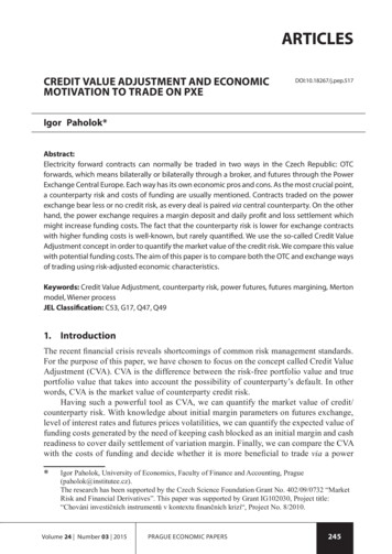
the electricity system in the Czech Republic1. More than 190 different contracts havebeen traded since the PXE founding.For the purpose of this essay, we need to examine the development of prices moreclosely. From the daily observed closing price we can calculate log returns, which wecan use for the calculation of contracts’ historical2 price volatility σ. As a quite largeamount of contracts has been traded since July 17, 2007, we have to aggregate contractsaccording their characteristics into six groups; base load and peak load months, quartersand years. Extended characteristics of contracts’ volatilities are presented in Appendix 1.Aggregated characteristics, which we use for CVA calculation, are listed in Table 1.Table 1 Characteristics of Historical Volatilities for Particular Contract GroupsContract type /Parameter1-percentile (%)Average (%)99-percentile (%)Margin (EUR)BL M0.010.811.874.5BL Q0.010.82.082.9BL Y0.010.711.362.7PL M0.010.832.057.5PL Q0.010.812.473.7PL Y0.010.821.553.5Source: PXE data, author’s analysisSubsequently we can use the obtained historical volatilities as a parameter forEquation 2.3 to simulate the paths of the Brownian motion and to evaluate the portfolioaccording 2.4. The usage of the Wiener process assumes the normality of daily returns.However, this assumption is arguable, we work with 190 time series with differentcharacteristics of returns distribution and therefore, the usage of a proxy distributionis inescapable. The illustration of the different returns distribution of PXE’s contractsis illustrated on Figure 1.In energy companies’ practice, a more sophisticated model than the Wiener processcould be used in the process of contract’s volatility modelling. The Two-Factors Model(see for example Ruediger, Schindlmayr, Reik (2005)), which incorporates the factthat the volatility of the contract increase with decreasing time to delivery, could bea suitable one. Unfortunately, we cannot apply such model in our case, as the contracts’characteristics have changed dramatically over time since 2007.At the end of this subsection, it has to be mentioned, that in the true sense of the wordthe market data from PXE are not necessarily from the market. Whenever the liquidity is1In the PXE, contracts with the delivery location within the electricity system in the Slovakia andHungary are also traded. We are concerned with Czech power futures in this paper, however, similarmethodology could be applied also to other countries.2Options for Czech power futures are not traded on the PXE. Therefore we cannot use impliedvolatilities.250PRAGUE ECONOMIC PAPERSVolume 24 Number 03 2015
low, and no contract is traded during the day, the exchange officer might adjust the endof day prices according particular exchange rules.Figure 1 The Illustration of Different Returns Distribution of PXE’s ContractsSource: PXE data, author’s analysis3.2 Euro interest rates data characteristicAccording to Equation 2.11 the funding costs depend on several interest rates of a particular currency which is the euro. Compared to OTC trades, the margin set by an exchangebears only the spot (overnight) rate minus the specific adjustment. The difference betweenthe longer term yield r(0,T) and the yield which bears margin deposit on an exchange rex isassumed to be the opportunity costs of the obligation to keep the margin deposit. However,if we trade rather OTC, we do not have to deposit a margin, and therefore, the particularamount could be invested. The duration of our alternative investment T equals the lengthof the period we intend to keep the position in the particular power futures contract.The second part of the defined funding costs is conditional. Whenever the end of dayvaluation, Vi(t), of contracts we hold in a position on an exchange, decreases under thevalue at the time of contracts initiating V0, we have to settle that negative mark-to-marketloss and vice versa. Anytime we open a position on an exchange, we have to take intoaccount the potential funding costs which arise from the obligation of the daily profit/losssettlement. This daily settlement is not common on OTC markets, and if our mark-tomarket position is negative, we do not have to settle it daily. The particular amount mighttherefore be invested in the overnight money market with the interest rON.Deposited margins on PXE bears an interest, which is calculated as the EONIA3minus 0.08 %. We suppose that we intend to keep position in the particular power futurecontract for a one year, therefore, we compare the PXE interest yield with the one-yeardeposit rate for the euro. The development of EONIA, the one-year euro deposit interest3Effective Overnight Index AverageVolume 24 Number 03 2015PRAGUE ECONOMIC PAPERS251
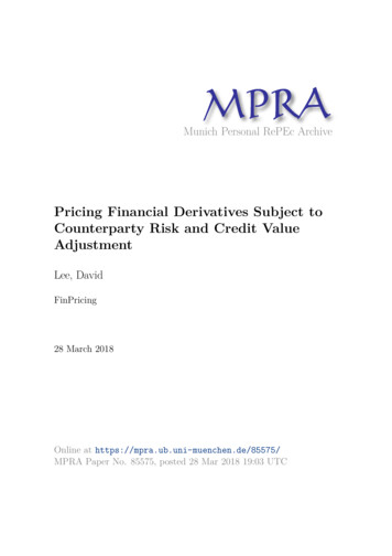
rate, the euro overnight interest rate, and the difference between one-year euro rate andthe rate paid by PXE for deposited margins since July 17, 2007 is presented in Figure 2.Figure 2 Development of Related Euro Interest RatesSource: ReutersAfter an overview of related interest rate development, it raises the question,which values of particular interest rates are supposed to be used in CVA and CriticalPD calculation. If we calculate CVA in a real business situation, we should apply anappropriate interest rate model, for example the Vasicek model, Cox-Ingersoll-Ross modelor Hull-White model, presented for example in Malek (2005). Historical data are used formodel calibration, and current values are used as initial values in the selected interest ratemodel. For a historical study as presented in this paper we use an average of historicalobservation and the critical values calculated as 1st and 99th percentile, presented in Table 2.This can be considered as historical simulation.Table 2 Characteristics of Historical Related Euro Interest RatesParameterr ONr(0,T)-rexr(0,T)1-percentile (%)Average (%)99-percentile (%)0.21.884.30.270.951.621.112.845.47Source: PXE data, author’s analysisThe results are also more objective than the results we would obtain if we used onlyvalues from the end of 2010.252PRAGUE ECONOMIC PAPERSVolume 24 Number 03 2015
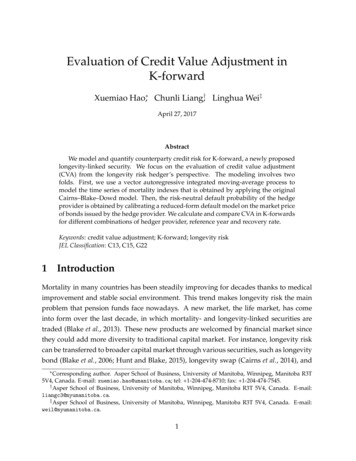
3.3 Modified Merton model and default probabilities calculationWe do not have historical observation about energy companies’ default probabilities.Instead of historical observation, we use the modified Merton model, as it was describedin Section 2.2. Using a predefined range of assets over debt ratio Y0 (1.08; 1.53) anda predefined range of assets over debt ratio volatility σY (0.002; 0.02) we obtain a rangeof realistic PD. Detailed PD distribution is presented in Appendix 2, graphically in Figure 3.Probability of defaultFigure 3 Default Probabilities Obtained from the Modified Merton ModelAsset over debt ratioDaily volatility of asset over debt ratioSource: Author’s analysis3.4 The CVA and critical PD calculationThe data described in the previous sections are just input parameters for the CVA andCritical PD calculation.The historical price volatilities presented in Table 1 are inputs for the portfolioconditional value calculation. We assume that the portfolio is always composed of onesingle contract. CVA is calculated for one MWh of this contract. The PDs are obtainedfrom the Modified Merton model and the recovery rate is set at 40%, which representsa market benchmark. The estimation of the recovery rate should be used in the firms’practice for each single counterparty. The average closing prices from December 31, 2010was set as the starting point X0 for each simulated time series, for each selected contracttype. The period for which we intend to keep the position is set as 250 working days.We do not consider either of the products cascading4, nor the delivery period.4On the accounting day following the last trading day for a particular year futures series, each openposition is replaced with an equivalent three month futures series (for January, February and March)and three corresponding quarter futures series (quarter for the second, third and fourth quarters).Each open position in the particular quarter futures series is replaced by an equivalent three monthfutures series.Volume 24 Number 03 2015PRAGUE ECONOMIC PAPERS253
The illustrative simulation for BL M time series with the average daily volatilityσ 0.81%; and the initial value EUR 49.75, is depicted in Figure 4. The portfolioconditional value is set as the 99th percentile of all 10,000 simulated paths. We usethe maximum of the conditional value series as an input for the CVA calculation.The maximum of the presented conditional portfolio value series is 66.51. Ourpotential exposure equals the positive mark-to-market value of our portfolio. This isgiven by the difference between the initial value of the contract and the conditionalvalue of the contract, which is EUR 16.75 for our example. This value is discounted withthe deposit rate for a particular tenure (the average of a one-year deposit rate is in ourcase 2.84%), multiplied by (1-RR), and finally, multiplied by PDs. The PDs are presentedin Appendix 2 and the relevant CVAs in Appendix 3. CVA, as it was mentioned before, isthe market value of credit risk which bears the counterparties in OTC trading.Figure 4 The Illustrative Simulation for the BL M Time SeriesSource: Author’s analysisThe funding costs contain two parts. The first one, cost of deposited margin, is calculatedas the opportunity cost of the obligated margin deposit. We calculate with a margin requirement of EUR 4.5 in our illustrative case for the BL M contract type. According to Equation 2.8we also calculate with the yield difference – 0.95%. For the calculation of the second fundingcost, we use the conditional value set as the 1st percentile of our stochastic simulation.The difference between the initial value of 1 MWh of electricity and the conditional Vt valueis multiplied by the related spot interest rate. As we use the average value in this case, wecalculate with the value rON 1.88%. The sum of both parts of the funding cost is finallydiscounted with the particular rate rtau to receive the present value of the money. Funding costsare EUR 0.16 in our illustrative example. As it was mentioned before, the funding costs arethe opportunity costs of electricity contracts traded via a power exchange.254PRAGUE ECONOMIC PAPERSVolume 24 Number 03 2015
The Critical PD, in other words, the probability of default for which it is economically irrelevant whether we trade via exchange or OTC is calculated as the PD for whichCVA equals the funding costs. In our case, we got the critical PD 1.6% which representsa company with a credit rating somewhere between Ba2 and Ba3 of Moody’s rating scale.If a counterparty has a rating or PD which is better than the critical value, we shouldtrade OTC. If the counterparty’s rating is worse than the critical, we should trade on anexchange.After the illustrative calculation, we reveal the results of the critical PDs value for allproduct types presented in Table 1. We calculate the characteristic for the average valuesof daily volatilities as well as for 99th percentile and 1st percentile. We use the averagevalues of the related interest rates from Table 2, for the funding costs calculations. Resultsof the described analysis is in the Table 3.Table 3 Values of the Critical PD for the Table 1 Contract Type Characteristics Data and Averageof the Related Interest Rate Data from Table 2Starting price(EUR)1st percentile(%)Average(%)99th percentile(%)Margin(EUR)BL M49.7539.591.601.054.5BL Q50.4427.131.490.972.9BL Y52.3524.221.531.132.7PL M61.9556.001.781.087.5PL Q63.127.041.440.823.7PL Y66.2524.901.451.143.5Critical PDSource: PXE data, author’s analysisThe critical PDs are very high for contracts with very low volatilities (around1st percentile of all contracts traded on PXE). Therefore it is more economical to tradesuch contracts OTC. The critical PDs for the contracts with the average volatilities ofeach contract type, varies from 1.44% to 1.78%. We get the highest values for the monthproducts, where the margin requirements are quite high. The critical PDs for high volatilitycontracts varies from 0.82% to 1.14%, which could be presented as the rating betweenBa1 and Ba2 on the Moody’s rating scale.The average values of the related interest rates are quite high compared to the interestrates of a post-crisis period. Therefore, we perform an analysis where we use the averagevalues of the contracts type volatilities of each contract type. But with the 1st percentileand 99th percentile of the related interest rate values as they are presented in Table 2.The results are in Table 4.Volume 24 Number 03 2015PRAGUE ECONOMIC PAPERS255
Table 4 Values of the Critical PD for the Table 2 Related Interest Rate Data and Averageof the Contract Type Characteristics Data from Table 1Starting price(EUR)1st percentile(%)Average(%)99th percentile(%)Margin (EUR)BL M49.750.251.603.634.5BL Q50.440.201.493.322.9BL Y52.350.211.533.502.7PL M61.950.291.783.867.5PL Q63.10.211.443.333.7PL Y66.250.201.453.253.5Critical PDSource: PXE data, author’s analysisIt is obvious that the critical PDs decrease dramatically when we use the low interestrate characteristics. For the period of very low interest rates the critical PDs implies Moody’srating around Baa2. Trading on the PXE is much more economical during the period withlow interest rates than during the period with a high level of related interest rates.4. ConclusionThe Credit Value Adjustment is a powerful tool, which allows us to quantify the marketvalue of credit/counterparty risk. Using this tool we can perform the analysis of theeconomic effectiveness of both types of trading; OTC and via exchange. The fundingcosts, which are typical for exchange trading, can be compared to the CVA, which isthe potential cost of OTC trading. The optimal way of trading can be recommended forthe various parameters as the counterparty’s default probability, the level of related interestrates, the volatility of traded instruments etc. Research shows how the critical probabilityof counterparty’s default (the default probability for which it is economically indifferentwhether we trade OTC or via exchange) varies with the different input parameters fromthe values around 50%, for the contracts with the very low volatility, to the values around0.2% which represents credit rating around Baa2, for the very low level of the relatedinterest rate values.The analyses presented above could be meant as an introduction to a more preciseanalysis on the energy trading company’s risk management level. The series of assumptionsand simplifications led to the indicated results. The real estimation of the recovery rateshould be performed for each counterparty (there is a significant difference whether wetrade with a small trading company or with a large power producer), the more suitablestochastic model for power contracts prices development should be applied as well asthe stochastic model for yield curve modelling. The existence of the so-called generalwrong way risk should be taken into account. General wrong-way risk is a term used todescribe possible sources of positive correlation between the exposure and the probabilityof default. The calculation with the wrong-way risk would probably increase the CVA,which could make trading via an exchange more economical. A more detailed researchof the CVA application in the energy sector is still required.256PRAGUE ECONOMIC PAPERSVolume 24 Number 03 2015 pa
For the purpose of this paper, we have chosen to focus on the concept called Credit Value Adjustment (CVA). CVA is the difference between the risk-free portfolio value and true portfolio value that takes into account the possibility of counterparty's default. In other words, CVA is the market value of counterparty credit risk. Having such a .