Transcription
HIGH POWER, REFLECTION TOLERANTRF SOLID STATE AMPLIFIER DESIGNByStephen Andrew ZajacA THESISSubmitted toMichigan State Universityin partial fulfillment of the requirementsfor the degree ofElectrical Engineering – Master of Science2013
ABSTRACTHIGH POWER, REFLECTION TOLERANT RF SOLID STATE AMPLIFIER DESIGNByStephen Andrew ZajacRF amplifiers have been developed for use in the Facility for Rare IsotopeBeams (FRIB) linear accelerator facility, which is currently under construction atMichigan State University. The development process has included the design, building,and testing of individual components, which together make a full-scale prototypesuitable for testing purposes.These full-scale prototypes can be used inSuperconducting Radio Frequency (SRF) resonator cavity conditioning, low energylinear accelerators such as the ReA3 re-accelerator, or simply bench tested.The design of an amplifier suited for driving a linear accelerator cavity is differentfrom an amplifier designed for more conventional applications such as FM or UHFbroadcasting in several ways. Most importantly, amplifiers used in linear acceleratorcavity applications are repetitively subject to full reflection load conditions which candestroy the amplifier in seconds. This necessitates the use of a circulator in everyamplifier. Accelerator cavities also require power levels in the 2 – 8 kW range, which issignificantly above what a single solid state power transistor can handle.Amplifier components discussed include pallet amplifiers, along with low passfilter circuits, circulators, and power combiner blocks. Together, these four componentscan be used to create an amplifier system which reaches the power levels required, cantolerate a full reflection load through all phases, and meets the longevity and costrequirements set forth by the FRIB project.
To my parents Tom and Susan.iii
TABLE OF CONTENTSLIST OF TABLES . viLIST OF FIGURES . viiCHAPTER 1INTRODUCTION . 11.1Power and Frequency . 71.2Device Technology . 91.3FRIB Specifications . 121.4Thesis Layout . 15CHAPTER 2PALLET AMPLIFIERS. 172.1Impedance Matching and Biasing . 182.2Circuit Design . 202.3Pre-Amp Pallets and Power-Amp Pallets . 212.4Amplifier Classes and Efficiency . 242.5Effects of Gate and Drain Biasing Voltages. 25CHAPTER 3LOW PASS FILTERS . 313.1Measured Performance . 32CHAPTER 4CIRCULATORS . 364.1Measured Performance . 394.2Temperature Dependence. 46CHAPTER 5POWER COMBINERS . 495.1TEE Combiner . 535.2Wilkinson Combiner . 545.3Hybrid Combiner . 54CHAPTER 6SYSTEM TESTING . 656.1Measurement Examples . 676.2Directional Couplers for High Power Measurements . 70CHAPTER 7CONCLUSION AND FUTURE WORK. 73iv
7.17.27.3Class H Amplifiers . 75Reflection Tolerant Transistors . 76Diamond Transistors . 77APPENDICES . 81APPENDIX A2 kW RF Amplifier Setup Procedure . 82APPENDIX BCirculator Testing Report: RF-Lambda RFC2101 SN:20110402. 93BIBLIOGRAPHY . 97v
LIST OF TABLESTable 1.1RF amplifier requirements for the FRIB project [5] . 12vi
LIST OF FIGURESFigure 1.1Chart of the Nuclides showing expected isotope production of FRIB. [5]For interpretation of the references to color in this and all other figures,the reader is referred to the electronic version of this thesis. . 2Figure 1.2Internal view of the K1200 cyclotron at MSU [5] . 4Figure 1.3Folded arrangement of the FRIB linear accelerator [5] . 5Figure 1.4200 kW vacuum tube amplifier final stage [5] . 6Figure 1.5Power vs. Frequency for solid state and vacuum based devices [9] . 9Figure 1.6Cross section of an LDMOS transistor [13] . 10Figure 1.7Layout of a 1 kW LDMOS device [13] . 11Figure 1.880.5 MHz (β 0.041/0.085) and 322 MHz (β 0.041/0.085)cavities [2] . 14Figure 2.1Impedance matching and biasing in an RF pallet amplifier . 17Figure 2.2Schematic of a 1 kW amplifier using an NXP BLF578 transistor . 19Figure 2.310 W 80.5 MHz pallet amplifier [17] . 22Figure 2.41 kW 80.5 MHz pallet amplifier [17] . 23Figure 2.5Gain vs. output power with a varying drain voltage . 27Figure 2.6Gain vs. output power with a varying gate voltage . 27Figure 2.7Output power vs. input power with a varying drain voltage . 28Figure 2.8Output power vs. input power with a varying gate voltage . 28Figure 2.9Third harmonic distortion vs. input power with a varying drain voltage . 29Figure 2.10Third harmonic distortion vs. input power with a varying gate voltage . 29Figure 2.11Efficiency vs. output power with a varying drain voltage . 30vii
Figure 2.12Temperature rise vs. output power with a varying drain voltage . 30Figure 3.17th order low pass filter, with a harmonic absorbinghigh pass filter [17] . 31Figure 3.2Insertion loss of a high power low pass filter. S21 -0.1 dB at322 MHz, and S21 -70 dB at 644 MHz . 33Figure 3.3Return loss of a high power low pass filter. S11 -20 dB at322 MHz, and S11 -0.5 dB at 644 MHz . 34Figure 3.4Harmonic content of a typical 1 kW Class C power amplifier . 35Figure 4.12 kW 80.5 MHz circulator. Input (left), output (right),isolation (top) [19] . 36Figure 4.2Characterizing circulator performance with a network analyzer . 37Figure 4.3Custom made 1 5/8” EIA short circuit used for testing circulators . 38Figure 4.41 5/8” EIA open circuit used for testing circulators . 38Figure 4.5Circulator insertion loss with a matched load on the output.S21 -0.7 dB at 80.5 MHz . 40Figure 4.6Circulator return loss with a matched load on the output.S11 -23 dB at 80.5 MHz . 41Figure 4.7Circulator return loss with an open circuit load on the output.S11 -35 dB at 80.5 MHz . 42Figure 4.8Return loss vs. output power for an in spec 80.5 MHz circulator . 44Figure 4.9Return loss vs. output power for an out of spec 80.5 MHz circulator . 44Figure 4.10Return loss vs. output power for an in spec 322 MHz circulator. 45Figure 4.11Temperature dependence of a circulator with anopen, short, and load . 46Figure 4.12Shift in return loss: circulator on metal stand (blue) vs. circulator onplastic stand (purple). 48Figure 5.14 kW TEE (top), 2 kW Wilkinson (bottom left), 8 kW hybrid(bottom right) . 49viii
Figure 5.2Loss vs. phase mismatch in a TEE combiner . 50Figure 5.3Results of a 2 kW Wilkinson combiner test . 51Figure 5.4Low power test setup for measuring a 4 kW 322 MHzhybrid combiner . 52Figure 5.5TEE combiner return loss. S11 -6.3 dB at 322 MHz. 56Figure 5.6TEE combiner insertion loss. S31 -2.8 dB at 322 MHz . 57Figure 5.7TEE combiner isolation. S21 -5.8 dB at 322 MHz . 58Figure 5.8Wilkinson combiner return loss. S11 -26 dB at 80.5 MHz . 59Figure 5.9Wilkinson combiner insertion loss. S31 -3.3 dB at 80.5 MHz . 60Figure 5.10Wilkinson combiner isolation. S21 -29 dB at 80.5 MHz . 61Figure 5.11Hybrid combiner return loss. S11 -32 dB at 322 MHz . 62Figure 5.12Hybrid combiner insertion loss. S31 -2.8 dB at 322 MHz . 63Figure 5.13Hybrid combiner isolation. S21 -33 dB at 322 MHz . 64Figure 6.1Test bench setup for measuring an amplifier using adirectional coupler . 65Figure 6.2Test bench setup for measuring an amplifier using adirectional coupler (2) . 66Figure 6.380.5 MHz 2 kW amplifier testing for the ReA3 reaccelerator . 68Figure 6.480.5 MHz 4 kW amplifier testing . 69Figure 6.5Amplifier test setup using a dual directional coupler andvector voltmeter . 70Figure 6.6Frequency response of an 80.5 MHz dual directional coupler.S21 -39.9 dB . 71Figure 6.7Spectral output of a directional coupler before accounting forresponse. 72Figure 7.1Thermal conductivity of diamond compared to copper and silicon [12] . 78ix
CHAPTER 1INTRODUCTIONOn December 11th, 2008, Michigan State University was selected over ArgonneNational Laboratory to construct the Facility for Rare Isotope Beams (FRIB) [1]. The550 million dollar facility was proposed almost 10 years ago, and will take another 10years to construct, but will significantly advance the field of rare isotope research.Michigan State University has been a leader in this field since the 1960s with theconstruction and continued growth of the National Superconducting CyclotronLaboratory (NSCL); however, the accelerator technology used in this facility is reachingits limits. When FRIB is finished near the end of this decade, it will completely replacethe front end of the current NSCL facility, while reusing much of the experimental space.To understand the need for a new accelerator, a brief overview of a few nuclear physicsconcepts is necessary.Figure 1.1 shows the expected isotope production of the FRIB facility in a formatreferred to as a “chart of the nuclides” [5]. The y-axis lists the number of protons in anatom, while the x-axis lists the number of neutrons. The number of protons determinesthe element; for example 6 protons results in the element carbon, while adding anotherproton results in the element nitrogen. Changing the number of neutrons in an atomdoes not change the element, but does change the atomic weight. Atoms with thesame number of protons but different numbers of neutrons are called isotopes, and areof great interest to nuclear physicists. Referring back to the chart of the nuclides, theatoms near the x y line are the stable isotopes that occur in nature and have lifetimes1
Figure 1.1: Chart of the Nuclides showing expected isotope production of FRIB. [5] Forinterpretation of the references to color in this and all other figures, the reader isreferred to the electronic version of this thesis.on the order of hundreds of years. Isotopes become harder to produce the farther onegets from the line of stable isotopes. The method that FRIB employs to create isotopesis to take a moderately stable heavy element such as uranium, accelerate it to abouthalf the speed of light, and smash it into a much lighter element (liquid lithium in thecase of FRIB). This is referred to as projectile fragmentation. The collision can breakup the uranium into several lighter elements, as well as add or subtract neutrons tocreate different isotopes. Accelerating an element such as uranium up to half the speedof light is not easy, and takes about 400 kW of beam power. The isotopes that arefarther away from the stable elements also have incredibly short lifetimes, on the orderof microseconds, making them extremely difficult to study. The chances of creating oneof these rare isotopes with a brute force approach like smashing atoms together is veryrare. The existing NSCL facility at MSU has run 24 hours a day for a week in certain2
experiments just to create one single copy of a rare isotope that would decay back to amore stable isotope in a matter of milliseconds. The result of this situation is thatisotopes closer to the stable elements are easy to produce in larger quantities, and thushave been studied extensively. Rare isotopes on the fringe of nuclear existence arevery difficult to produce in larger quantities, and thus very little is known about theirproperties. The main goal of FRIB is to study these rare isotopes.The accelerator used in the existing NSCL facility uses two superconductingcyclotrons connected in series to reach about half the speed of light [3].Thesecyclotrons are fairly compact and can fit in a 20 foot x 20 foot room, but their combinedpower usage is over a megawatt. The approach here is to use a small number of veryhigh power accelerators to reach the desired power level. The current NSCL facility canreach power levels close to what is being proposed in FRIB, however there is afundamental limit of cyclotrons that prevents them from creating large numbers of rareisotopes.A cyclotron works by injecting an atom into the center of three copperelectrodes (called dees) that are fed with an RF source that is 120 degrees apart oneach dee [4]. The injected atom will rotate in a circle around the interior of the cyclotronin sync with the applied electric filed. With each trip around the cyclotron the injectedatom will gain energy, increasing the radius of the circle in which it spins, and moving ittowards the outer edge. The atom will have gained full power once it reaches this edge,3
Figure 1.2: Internal view of the K1200 cyclotron at MSU [5].and it is then extracted and sent down the beamline towards the target. While the atomis in the cyclotron it makes a few thousand closely spaced rotations as it gains energy.The limitation of a cyclotron is in the number of atoms that can be packed into it at thesame time. This limits the so called beam current of the cyclotron, and means thatthere are less rare isotopes available for study.FRIB will employ the use of a linear accelerator, which has a different set oftradeoffs when compared to a cyclotron accelerator. While a cyclotron is a compactdevice that only requires one or two units to reach the desired power levels, a linearaccelerator uses hundreds of lower power accelerators that are connected in series toreach the desired power levels. Refer to figure 1.3 to get an idea of the scale of the4
Figure 1.3: Folded arrangement of the FRIB linear accelerator [5].FRIB linear accelerator [5]. The original plan had the entire facility running in a straightline of over 1000 feet, crossing Bogue St and starting out at McDonnell Hall. Thisapproach was abandoned in favor of the paperclip arrangement shown above, not onlybecause of simpler construction costs, but also because the two folding segments ateither end provide an opportunity to separate out different elements produced by the ionsource in relation to their weight. This configuration also allows closer spacing of thesupport facilities above ground.The challenge from an electrical engineer’s point of view is going from the 6amplifiers (3 per cyclotron, and 1 per dee) of the NSCL accelerator, to the hundreds ofamplifiers required for the FRIB accelerator. The amplifiers used in the cyclotron arevaried between 10 MHz and 20 MHz based on the element being accelerated, and havepower levels in the 100 to 200 kW range. These amplifiers are very similar to what isused in over-the-air broadcasting (FM and VHF bands), and use multiple vacuum tube5
Figure 1.4: 200 kW vacuum tube amplifier final stage [5].stages in cascade to reach the desired power levels. The final stage in a 200 kWvacuum tube amplifier is almost always water cooled, and the inlet to outlet watertemperature difference can be as high as 60 F with a flow rate of 30 gallons perminute. The amount of heat that these amplifiers must endure is enormous.While a vacuum tube based amplifier is good for reaching very high power levelsabove 100 kW while maintaining an acceptable efficiency of 50 – 60%, these systemsare very expensive to maintain, requiring frequent and costly tube replacement. WithNSCL, the solution was to keep replacement tubes in stock, and swap them out duringscheduled downtime to prevent an amplifier from going offline while an experiment was6
being run. This is very costly, but the alternative is several days of downtime for anunexpected repair on a facility that costs 20 million each year to run. FRIB will requireseveral hundred amplifiers in the 2 - 8 kW range at 80.5 MHz and 322 MHz [5]. Whilevacuum tube amplifiers exist in these power and frequency ranges, the downtime in afacility such as FRIB would be unacceptable. NSCL currently employs 2-3 full timetechnicians to maintain the cyclotron vacuum tube amplifier systems.Multiply thenumber of amplifiers used by 100, and it is clear that not only cost, but also labor wouldbe prohibitive.The lifetime of a solid state amplifier is measured in hundreds of thousands ofhours, compared to the lifetime of a vacuum tube amplifier which is measured inthousands of hours.The only problem with solid state amplifiers is that presentlyavailable RF transistors are only capable of output power levels around 1 kW [6], whileFRIB requires amplifiers in the power range of 2 – 8 kW.1.1 Power and FrequencySolid state transistors with cutoff frequencies approaching the THz band havebeen demonstrated [7] [8], but the power levels obtained are very small, on the order of1 mW. On the other extreme, single solid state transistors used for conversion of 60 Hzpower are available with power levels on the order of 10 kW [9]. The challenge is increating a device that is capable of both high power and high frequency.Thefundamental limits in play here are capacitance and thermodynamics.In order to create higher frequency devices, the dimensions must shrink toreduce the capacitance between the three terminals of the transistor. The impedance of7
a capacitor decreases as the frequency is raised, so above a certain frequency theeffective capacitance between the gate and the source of a transistor looks like a shortcircuit [10].Larger transistors have more surface area between the gate and thesource, and thus more capacitance, which lowers the maximum operational frequencyof the device.Creating a high power device is based on two factors: efficiency andthermodynamics. Any input power from the DC source that is not converted to RFpower at the output is converted to heat which is dissipated in the transistor.Forexample, a 1 kW transistor that is 67 % efficient will dissipate 500 W of heat in thetransistor. The present limit on how much heat can be removed from a power transistor2package while staying within safe operating temperatures is about 200 W/cm . Theeasiest way to get more power out of a transistor then is to increase the efficiency.Taking the previous example of a transistor that is 67 % efficient and somehowincreasing that to slightly above 80 % would result in only 250 W dissipated in the samearea, and could technically double the output power of the transistor if cooling was theonly barrier to higher power.The other options for getting more power out of atransistor are to increase the thermal conductivity of the heatsink, or even the materialthat the device itself is made of. Different transistor materials can also have highertemperature safe operating limits. Above about 200 C in silicon, thermal runaway andbreakdown occur which will melt the device [11].8
1.2 Device TechnologySolid state devices are mainly constructed from silicon, but other materials suchas GaN and SiC can also be used [9]. Likewise, there is a standard vacuum tube basedamplifier, along with other variants that have different power and frequencyspecifications, such as klystrons and gyrotrons. New device structures such as theLaterally Diffused Metal Oxide Semiconductor (LDMOS) have been used to push thepower levels that can be obtained with silicon from the 10-20 W as shown in figure 1.5to around 1 kW. This has been achieved even with the thermal conductivity and safeoperating temperature limits of silicon. Switching to another device technology couldtheoretically enable even higher power levels than this in a single transistor. The idealtransistor material would be crystalline diamond, which has a thermal conductivity atFigure 1.5: Power vs. Frequency for solid state and vacuum based devices [9].9
room temperature higher than that of copper, and a safe operating temperature severalhundred degrees above that of silicon [12]. Up until this point though, no one hasmanaged to successfully create a commercially viable transistor based on diamond dueto cost and manufacturing complexity.Silicon Carbide (SiC) devices are currentlyavailable, and offer operating temperatures significantly above that of silicon. Thesedevices are capable of 10s of kW, but are targeted towards 60 Hz power conversionapplications [9]. GaN based devices are available for high frequencies approaching theFigure 1.6: Cross section of an LDMOS transistor [13].10
THz frequency range, but output power is limited [9]. When comparing the high power,high frequency landscape, vacuum tube based amplifiers still dominate.Figure 1.6 shows the cross sectional area of an LDMOS transistor [13]. The keydetail to notice here is the separation between the drain and the source. This enables2higher voltage operation, which reduces the I R losses that heat up the device andreduce maximum power output. LDMOS technology has gone from 32 V devices, to thepresent 50 V devices, and 100V devices from ST Microelectronics are just starting to hitthe market.The other technique used in LDMOS transistors to increase the maximum poweroutput is shown in figure 1.7 [13]. Several device fingers are put in parallel to increasethe surface area available for cooling, and reduce the heat load on any one transistor.In a present state of the art silicon LDMOS transistor, the device area is about 1 cm by3 cm [6]. At a power level of 1 kW and an efficiency of 67%, this translates to a heat2load of about 500W, which is just under the thermodynamic cooling limit of 200 W/cm .Figure 1.7: Layout of a 1 kW LDMOS device [13].11
1.3 FRIB SpecificationsThe amplifier requirements for the FRIB project are shown in table 1.1 [5]. Theamplifiers designed were for the β 0.041 through β 0.530 cryomodules, along withthe matching cryomodules. This means the total number of high power RF solid stateamplifiers needed is 344. The 6 buncher amplifiers at the front end of the beamline willbe implemented used readily available 100 W solid state amplifiers, and the 200 kWRadio Frequency Quadrapole (RFQ) amplifier will use a vacuum tube based designsimilar to what was shown in figure 1.4.The β of a cryomodule refers to the speed of an incoming particle with respect tothe speed of light [14]. A cryomodule is simply a group of superconducting acceleratorcavities that are connected to the same cryogenic cooling system, typically 6 to 8. A βvalue of 0.530 at the end of the linear accelerator means that the particles are travelingat about half the speed of light, while a β of 0.041 means the incoming particles aretraveling at about 4.1% of the speed of light.The general operation of a linearaccelerator is as follows: an ion source at the front end of the accelerator creates aComponentQty# Cavities eachkW each# AmplifiersMulti-Harmonic BuncherEnergy EqualizerRebuncherRFQβ 0.041 Cryomoduleβ 0.085 Cryomoduleβ 0.285 Cryomoduleβ 0.530 CryomoduleMatching 024484312116967814410351Table 1.1: RF amplifier requirements for the FRIB project [5].12
charged beam of particles that can be manipulated by EM fields. This is a DC beamthat is then formed into packets to be accelerated using the buncher cavities. Thespacing is dependent on the design frequency of the accelerating cavities andamplifiers. This is 80.5 MHz for the β 0.041 and β 0.085 cavities, and 322 MHz forthe β 0.285 and β 0.530 cavities [5]. At this point the particles are traveling veryslowly. The RFQ is the first stage that imparts a significant amount of energy into thebeam.It also aids in focusing the beam for the upcoming accelerator stages.Defocusing of the beam is more of a problem in the initial stages, while it becomes lessof an issue at higher speeds [15]. After the RFQ, each of the 344 accelerating cavitiesgives a kick to the beam of particles, gradually increasing its speed from 4.1% of thespeed of light at the start, to 53% of the speed of light at the finish. The change inspeed is gradual, so a β 0.285 cavity for example can accept particles with a β /50%. It is most efficient at the designed β value, but having four standardized cavitydesigns reduces the manufacturing complexity [16]. After the last accelerating cavity,the beam of particles is sent towards the target where it is smashed against a film ofliquid lithium. The hundreds of isotopes that result are then sorted by charge and massand sent to the experimental area for study.The design considerations for a solid state amplifier are the frequency: 80.5 MHzor 322 MHz, the power levels required, and the load conditions that will be seen by theamplifier. Frequency and power requirements are relatively straight forward, but theload conditions can be a challenge. Figure 1.8 shows the basic design of an 80.5 MHzSuperconducting Radio Frequency (SRF) cavity, and a 322 MHz SRF cavity [2]. Thesecavities can be thought of as a basic EM resonator that holds energy in the form of13
Figure 1.8: 80.5 MHz (β 0.041/0.085) and 322 MHz (β 0.041/0.085) cavities [2].alternating electric and magnetic fields. By making the cavities superconducting, thelosses in the walls of the cavities are reduced to almost zero, and the cavity can store avery large amount of energy. When a bunch of particles comes along, most of thisenergy is transferred to the beam, and the stored energy in the cavity is emptied. Whenmore energy is being put into the cavity, this is an ideal load condition from the point ofview of the RF amplifier.Most of the power coming from the amplifier is beingtransferred to the cavity, and very little is being reflected back. However, when thecavity is full of energy, most of the power from the amplifier is reflected back. So apower transistor that was designed to handle 500W of heat could now see up to 1.5 kWof heat. This is a major issue that must be accounted for in the design of these RF solidstate
Figure 2.12 Temperature rise vs. output power with a varying drain voltage . 30 Figure 3.1 7th order low pass filter, with a harmonic absorbing high pass filter [17] . 31 Figure 3.2 Insertion loss of a high power low pass filter.