Transcription
Trend-Following Strategies in Futures MarketsA MACHINE LEARNING APPROACHArt PaspanthongDivya SainiJoe TaglicRaghav TibrewalaWill Vithayapalert1
Outline Overview of Data and Strategy Feature Generation Model Review› Linear Regression› LSTM› Neural Network Portfolio Results Conclusion2
Overview of Data andStrategy3
Our TaskProblem Statement:Replicate and improve on the basic ideas of trend following.4
DatasetsDatasets of Commodities FuturesEnergyMetalsAgricultureTotal Assets ConsideredCrude OilGoldCorn42 Different AssetsSilverWheatCopperTime Frame: 1 - 6 months ExpirationSoybeanFilteredout byliquidityTotal Assets TradedSource: Quandl36 Different Assets5
Data ExplorationVolatility PlotCorrelation Plot6
Data ExplorationGold 6-Month FuturesSell SignalWeak/FalseSignalBuySignal7
StrategyTraditional Trend FollowingNot about predictionInvolves quickly detecting a trend and riding it, all while managing when to exit at the right momentOur ApproachUse traditional trend following indicators to predict returns with machine learning techniquesUse a portfolio optimizer to weight assets using the predicted returnsAdhere to traditional investment practice with stop-loss8
Feature Generation9
Trend-following FeaturesContinuous}Simple Moving Average (SMA) with 5, 10, 15, 20, 50, 100 days lookback windowExponential Moving Average (EMA) with 10, 12, 20, 26, 50, 100 days lookback windowMoving Average Convergence Divergence (MACD) 12-day EMA - 26-day EMAMomentum Indicator with 5, 10, 15, 20, 50, 100 days lookback windowDay Since Cross indicates the number of days since crossoverNumber of days ‘up’ - ‘down’ with 5, 10, 15, 20, 50, 100 days lookback windowResponseNext Day Return [ Pt 1 - Pt ] / PtCategoricalSMA Crossover indicator variablesEMA Crossover indicator variablesMACD Crossover indicator variables( 1 crossover with buy signal, 0 no crossover, -1 crossover with sell signal)10
Model Review11
Model ReviewLinear Regression12
Linear Regression ModelUse a linear regression (ordinary least squares) for each asset on the available training dataAdvantages:Simple, easy to understandFits decently well to linear dataDisadvantages:Overfits easilyCannot express complex or nonlinear relationshipsPortfolio over 2017-2018Train MSE: 2.187 E-04Test MSE: 1.47 E-04Plot of Predicted vs. Actual Values and Error Histogram for Linear Regression, daily return13
Linear Regression ModelCovariate NameBeta ValueP ValueEMA 104.84.004EMA 202.45.219SMA 1000.06.004EMA 1000.03.17SMA 150.01.817SMA 10-0.002.981SMA 20-0.008.866SMA 50-0.04.149SMA 5-0.070.044EMA 50-0.29.235EMA 26-0.45.749EMA 12-6.38.016 Exponential Moving Averages aregenerally better predictors than simplemoving averages Recent trends are most significant Change of sign between EMA 10, 12,20 suggests importance of recentcrosses Significance of longest-range featureshows importance of long-termtrendiness14
Linear Regression Model with LassoLasso Regularization gets rid of some of the overfitting of a linear regressionAccomplished by automatically selecting only more important featuresAdvantages:Less likely to overfitLess prone to noiseDisadvantages:Does not solve complexity issueCan lose expressivenessPortfolio over 2017-2018Train MSE: 2.281 E-04Test MSE: 1.353 E-04Predicted vs. Actual values and Error Histogram for Lasso Regression, Daily Returns15
Linear Regression Model with 5-Day ReturnsDetermine whether the model can better predict returns over a longer time frameWhy is this desirable?In a non-ideal trading system there are frictions:One-day returns are small and may be erased by transaction costsMight not enter the position until the next dayCan we reliably predict 5-day returns?5-day returns are generally about 2-3x larger than 1 day returns, so a roughly 6.5x increase in meansquared error (MSE: 9.47E-04) indicates that the predictions are about equivalent to 1-day predictions.Interestingly, the daily returns of this portfolio vs. the naive portfolio arefairly comparable ( 0.04 % vs. 0.02% ) but the 5-day returns are notablybetter (0.22% vs. 0.07%).Plot of Predicted vs. Actual Values16
Model ReviewRNN: LSTM Model17
Long-Short Term Memory (LSTM) ModelArchitecture: 3-layer LSTM and one fully-connectedlayer with linear activation functionRegularization: Dropout, Early Stopping, GradientClippingHyperparameter Tuning: Select the best set ofhyperparameters includingBatch Size: 32, 64, 128 Lookback window 5, 10, 15 daysOptimizer: AdamStatistical Results:Daily ReturnMSE: 0.00031Correlation: -0.0165-day ReturnMSE: 0.0011Correlation: -0.25Dataset too small for LSTM to capture the“trend” and perform well18
Long-Short Term Memory (LSTM) ModelStatistics and VisualizationsNext Day’s ReturnPrediction on further returns is lessaccurate and more variantNext 5-Day’s Return19
Model ReviewNeural Net20
Neural Net ModelArchitecture: One input layer with 26 input units, twohidden layers with RELU activation functions and one outputlayer. The neural network is fully connected.Features Used: A total of 26 input features, given below: Normalized Simple Moving Average with 5, 10, 15, 20, 50, 100days lookback windowNormalized Exponential Moving Average with 10, 12, 20, 26, 50,100 days lookback windowNormalized Moving Average Convergence DivergenceCrossover dataStopping Criterion: The validation dataset is used forstopping. When the loss difference over the validation setdecreases below the convergence error, we stop thetraining.Hyperparameters: Learning Rate: 1e-3Convergence Error: 1e-6Number of units in hiddenlayers: 50 and 20respectivelyOptimizer: Adam21
Neural Net ModelDifficulty: The neural net model uses random initialization of the parametersand uses an iterative process (gradient descent) to find the minima. Thestochastic nature of the model gives us different results on running the model.For example, we have these three plots which run the same neural networkcode but gave us different results:22
Neural Net ModelComparison with Linear Regression The linear regression model gives the same result everytime but the neural network without activations (whichperforms simple gradient descent) does not give thesame result every time. The neural network has been given validation data andthe model stops training based on the validation loss,however, the linear regression can theoretically overfitthe past data. Sometimes the neural network (without activations)performs better than linear regression but sometimesworse. The MSE for linear regression and neuralnetwork (without activations) is almost equal. LRNNHowever, with RELU activations, it performs worsebecause of the nature of the data and the nature ofRELU.23
Neural Net ModelStatistics and VisualizationsFor comparison with the other models, we have used one of neural network models that we trained. Thestatistics and visualizations for that model have been shown below.Correlations between all results andall predictionsHistogram of errorsNeural network model with portfoliooptimization24
Results SummaryModelsMSE on train setMSE on test setLinear Regression2.187 E-041.47 E-04Lasso Model2.281 E-041.353 E-04Neural Net2.329 E-041.358 E-04LSTM1.34 E-033.05 E-0325
Portfolio Results26
Portfolio Optimization Calculate expected returns using model of choiceCalculate covariance matrix using historical dataDetermine desired variance based on a benchmark Usually an equal-weight long-only portfolioObjective: max expected portfolio return after transaction costsConstraints:Note: Covariance Shrinkage Transformed the samplecovariance matrix usingLeDoit-Wolf Shrinkage Mathematically: pulls the mostDoes not leverage portfolioExpected variance below desired varianceCurrent HoldingsExpected ReturnsObserved CovarianceDesired VarianceTransaction Costsextreme coefficients towards morecentral values, thereby systematicallyreducing estimation error Intuitively: not betting the ranch onnoisy coefficients that are too extremeTradesNew Holdings27
Baseline StrategyTraditional Trend FollowingBacktesting ResultEnter a position based on crossovers1 and/orbreakouts2(1) Crossover: Crosses between moving averages and actualprice of the asset(2) Breakout: When the price of the asset breaks out from therange defined by support and resistance lineOur Baseline Strategy Equal allocation to each assets Trading using crossovers Utilizing both non-moving stops andtrailing stopsSharpe Ratio: 1.494Annualized Profit: 3.815%Maximum Drawdown: -0.4134%28
Best TM0.14341.351%-4.360%29
Trading Costs and Stop LossTrading costs represented as a constant percentage of our trade size25 bp (0.25%) as a rough estimate (equities trade at 15 bp1)For each position, if the asset has a loss greater than x% since opening that position, close the positionStop losses at 15%, 10%, and 5% loss shown below, all seem to have a negative impact on portfolio.The losses we experience are typically not gradual, but sudden, and thus the stop loss is ty-commission-rates-remain-steady/30
Final ResultsLook at 2019 data as a small secondary test set, for a selected strategyUse Linear Regression and account for trading costs, without using a stop lossThe results are not exactly encouraging:The portfolio spends almost all year in the red compared to the simple allocation strategyWhere before the errors were more balanced, they are now distinctly more often negativeThe regression has several large mistakes that cost it significantly31
Conclusion32
Conclusions Simple Trend Following has the largest Sharpe ratio Learned models did not capture the logic behind trend following Accuracy doesn’t necessarily improve performance Stop loss did not improve performance of modeled strategies33
Future Work Data Collection: Larger Datasets To better facilitate deep learning models Seek a larger universe of assetsFeatures: Introducing new features Adding fundamental features (P/E, ROE, ROA, etc.) Adding more technical indicatorsModel: Develop the models for more accurate predictions Better tuning parameters: Random Search and Bayesian OptimizationBacktesting: Using test sets with tail events Our current test set (Year 2017 - 2018) is quite ‘typical’34
Questions?35
Trend-following Features Continuous Simple Moving Average (SMA) with 5, 10, 15, 20, 50, 100 days lookback window Exponential Moving Average (EMA) with 10, 12, 20, 26, 50, 100 days lookback window Moving Average Convergence Divergence (MACD) 12-day EMA - 26-day EMA Momentum Indicator with 5, 10, 15, 20, 50, 100 days lookback window Day Since Cross indicates the number of days since