Transcription
Circuit NoteCN-0507Devices Connected/ReferencedCircuits from the Lab reference designsare engineered and tested for quick andeasy system integration to help solve today’sanalog, mixed-signal, and RF designchallenges. For more information and/orsupport, visit www.analog.com/CN0507ADF4355-3Microwave Wideband Synthesizer withIntegrated VCOADL5380400 MHz to 6 GHz QuadratureDemodulatorHMC1044Programmable Harmonic Low-Pass Filter,1 GHz to 3 GHz, 3 dB BandwidthHMC8038High Isolation, Silicon SPDT, NonreflectiveSwitch, 0.1 GHz to 6.0 GHzHMC788ApHEMT Gain Block MMIC Amplifier, DC10 GHzADG739CMOS, Low Voltage, 3-Wire, SeriallyControlled, Dual-SP4T SwitchAD8426Wide Supply Range, Dual, Rail-to-Rail,Output Instrumentation AmplifierADR127Precision, Micropower LDO VoltageReferences in TSOTADM7150800 mA Ultralow Noise, High PSRR, RFLinear RegulatorADM71726.5 V, 2 A, Ultralow Noise, High PSRR, FastTransient Response CMOS LDOA Complete Two-Port Vector Network AnalyzerEVALUATION AND DESIGN SUPPORTCircuit Evaluation Boards2-Port Network Analyzer Board (EVAL-CN0507-ARDZ)Ultra low power ARM Cortex-M3 Arduino Form FactorDevelopment Platform (EVAL-ADICUP3029)Design and Integration FilesSchematics, Layout Files, Bill of Materials, SoftwareCIRCUIT FUNCTION AND BENEFITSVector network analysis is a technique to measure the phaseshift and attenuation of signals as they propagate through amedium or are reflected by the medium. This technique is mostcommonly used to measure the gain, reflection coefficient, andreverse isolation of electronic circuits, such as RF amplifiers andfilters, but can also be expanded to analyze characteristics of amaterial, such as its moisture content.The reference design shown in Figure 1 implements a completetwo-port radio frequency (RF) vector network analyzer using azero intermediate frequency (ZIF) architecture. The frequencyrange of the circuit is from 1.7 GHz to 3.4 GHz, and thedynamic range is approximately 40 dB.Directional couplers and in-phase-quadrature (IQ)demodulators sense the forward and reverse phase andamplitude. Because of the zero IF architecture, the IQdemodulator outputs are at dc and can be sampled directly by aprecision analog-to-digital converter (ADC) integrated into amicrocontroller.A major advantage of the reference design is the use of the ZIFarchitecture, where use of a lower speed ADC reduces cost andavoids the design complexity associated with high speedsampling converters. This architecture enables the CN-0507board to be compatible with low cost Arduino form factorboards and provides users with an alternative to bulky,expensive benchtop lab equipment that can cost thousands ofdollars. The compact size of the reference design makes it idealfor a wide range of test and measurement applications.Rev. 0Circuits from the Lab circuits from Analog Devices have been designed and built by Analog Devicesengineers.Standard engineeringpractices havebeen employedin the design and construction of eachcircuit, and their function and performance have been tested and verified in a lab environment at roomtemperature. However, you are solely responsible for testing the circuit and determining its suitabilityand applicabilityfor youruse and application. Accordingly,in no event shallAnalog Devicesbeliablefordirect, indirect, special, incidental, consequential or punitive damages due to any cause whatsoeverconnected to the use of any Circuits from the Lab circuits. (Continued on last page)One Technology Way, P.O. Box 9106, Norwood, MA 02062-9106, U.S.A.www.analog.comTel: 781.329.4700Fax: 781.461.3113 2020 Analog Devices, Inc. All rights reserved.
CN-0507Circuit NoteHMC8038SPDT50Ω122.88MHzEXTREFHMC8038SPDTTO ANALOG MUXI2RQ2RIQ DMODADL5538050ΩPORT2HMC1044PROGRAMMABLELPFRFOUT A50Ω50ΩIQ DMODADL55380Q2FI2FTO ANALOG MUXDUTORMUTTO ANALOG MUXADF4355PLL WITHINTEGRATEDVCOI1RHMC1044PROGRAMMABLELPFRFOUT BQ1RIQ DMODADL55380HMC788GAINBLOCKPORT 11-TO-4POWERSPLITTERIQ DMODADL55380I1FANALOG MUX IADG739I1FQ1FTO ANALOG MUXIN AMPAD8426TO AIN CONNECTOR(ADICUP3029)I1RI2FI2RANALOG MUX QADG739Q1FVREFADR127IN AMPAD8426Q1RVQ23361-001Q2FQ2RFigure 1. Simplified block Diagram of EVAL-CN0507-ARDZCIRCUIT DESCRIPTIONAnalysis of a Linear NetworkAt RF, analysis of a linear network is executed using powerwaves, which can be related to the traveling voltage and currentwave phasors. The scattering, or S-parameters, are the mostcommon quantities to describe the electrical behavior of thenetwork at high frequencies. The term, scattering, refers to theway the electromagnetic (EM) wave is affected as the wavepasses a discontinuity.b1b2PORT 1PORT 2a223361-002a1Figure 2 shows a two-port network with four traveling voltagewave phasors that are defined as follows:a1 is the incident wave at Port 1b1 is the reflected wave at Port 1a2 is the incident wave at Port 2b2 is the reflected wave at Port 2The four S-parameters of the network are defined asS11 b1, the forward reflectiona1 S21 b2, the forward gaina1 S12 b1, the reverse isolationa2 S22 b2, the reverse reflectiona2A vector network analyzer measures the voltage wave phasorsand computes the S-parametersTraditional Network Analyzer ArchitectureFigure 2. S-Parameters Figure 3 shows the architecture of a traditional network analyzer,configured to measure dual-port S-parameters. Phase-LockedLoop 1 (PLL1) drives a sine wave into one of the two ports ofthe network, while the other port is internally terminated to50 Ω. The device under test (DUT) or material under test(MUT) is generally connected between the RF ports (a MUTsample is placed between two antennae connected to the twoports).Rev. 0 Page 2 of 13
Circuit NoteCN-0507sampled by baseband ADCs (such as successive approximation(SAR) and low speed sigma delta (Σ-Δ architectures) ratherthan with IF sampling ADCs.While PLL1 conducts a stepped frequency sweep, portions ofthe incident, transmitted and reflected signals, are coupled offby four in-line directional couplers. These directional couplersdrive four mixers that down convert the signals to a lowintermediate frequency (IF). The local oscillator (LO) inputs ofthe four mixers are driven by a second PLL (PLL2).PORT2For the intermediate frequency to remain constant, PLL1 andPLL2 need to track each other with a small offset frequencyequal to the IF. This offset is usually a few hundred kHz.50ΩADC ADCADC ADCADC ADCADC ADCPLL150ΩWith the absorptive single-pole double-throw (SPDT) switch inthe position shown in Figure 3, PLL1 drives Port 1 and Port 1 isterminated to 50 Ω. With the amplifier under test connected asshown (input connected to Port 1), the sweep yields data that isused to calculate S11 (input reflection) and S21 (gain). By flippingthe SPDT to its other position, PLL1 drives Port 2, yielding thedata required to calculate S22 (output reflection) and S12 (reverseisolation).PORT2DUTORMUTPORT 123361-004The circuit is completed by four IF sampling ADCs. The ADCoutputs are digitally downconverted to baseband to yieldamplitude and phase vectors. The S-parameters of the DUT orMUT are the ratios of these vectors.Figure 4. A Zero IF based Network AnalyzerThe ADF4355-3 PLL offers high output power, a widefrequency range, and dual outputs. In addition to providing thedrive signal to the active port, the ADF4355-3 also provides LOdrive for the four IQ demodulators.The main signal path (starting at RFOUTA), as shown in Figure 5,consists of a programmable low-pass filter (HMC1044), a balun,two HMC8038 absorptive SPDT switches, and a bidirectionaldirectional coupler.50Ω50ΩADCPLL2ADCThe HMC1044 filters the harmonics of the output signal of thePLL. The corner frequency of the HMC1044 must therefore beadjusted during the frequency sweep of the PLL. The first SPDTswitch provides signal isolation during the dc offset calibrationroutine and the second SPDT switches the signal to either Port 1or Port 2.DUTORMUTADCPORT 123361-003ADCPLL1Figure 3. Core Elements of a Network AnalyzerZero IF ArchitectureAn alternative approach is shown in Figure 4 in which themixers are replaced with IQ demodulators and a single PLL isused to drive the DUT and the LO inputs of the IQ demodulators.This result yields baseband IQ vectors directly at the outputs ofthe IQ demodulators. Because the IQ demodulator outputs areat dc (while the PLL is at a particular frequency), the outputs beThe bidirectional couplers have a coupling factor ofapproximately 15 dB and provide coupled forward and reversesignals to the four ADL5380 wideband IQ demodulators. Thedc outputs of the four IQ demodulators are multiplexed downto a single pair of IQ signals by two ADG739 CMOS switches.Finally, these differential signals are applied to two AD8426instrumentation amplifiers that convert the differential signalsto single-ended signals with a dc offset of 1.25 V set by theADR127 voltage reference. At this point, these two signals arerouted to the standard analog input Arduino connector to besampled by the integrated 12-bit ADC on the ADuCM3029.Rev. 0 Page 3 of 13
CN-0507Circuit NoteHMC8038SPDT50Ω122.88MHzEXTREFHMC8038SPDTTO ANALOG MUXI2RQ2RIQ DMODADL5538050ΩPORT2HMC1044PROGRAMMABLELPFRFOUT A50Ω50ΩIQ DMODADL55380Q2FI2F50ΩTO ANALOG MUXTO ANALOG MUXI1RQ1RADF4355PLL WITHINTEGRATEDVCOHMC1044PROGRAMMABLELPFRFOUT BIQ DMODADL55380HMC788GAINBLOCKPORT 11-TO-4POWERSPLITTERI1FANALOG MUX IADG739I1FSCLK AND ENABLEPOWERMANAGEMENT 6VDUTORMUTLDOREGULATORADM7172LDOREGULATORADM7150 5V 3.3VDIO H FROMADICup3029DIO L FROMADICup30291234567891012345678I1RTO AIN CONNECTOR(ADICUP3029)I2FI2RQ1FS21S11TO ANALOG MUXIN AMPAD8426ANALOG MUX QADG739IQ DMODADL55380Q1FVREFADR12712345678A0A10V TO 2.5VIN AMPAD8426Q1RVQ23361-005Q2FQ2RFigure 5. Block Diagram with Signal Flow for Measurement of S11 and S21The LO drive path (RFOUTB) also includes the HMC1044programmable low-pass filter to reduce LO harmonics. Thisfilter is followed by a balun, an HMC788A broadband gainblock, and a passive 1-to-4 power splitter (built discretely on theboard using resistors).The availability of two synchronized but independent PLLoutputs has multiple benefits. While the output power of the LOdriving output (RFOUTB) is held steady, the output power levelfrom RFOUTA (which drives the DUT or MUT) can be variedover a range of approximately 10 dB. This feature can be used tomaximize dynamic range based on the application. Forexample, when measuring a passive device or material, thepower level on RFOUTA can be set to its maximum. Incontrast, when measuring an active device with gain, such as anRF amplifier, the PLL source power can be backed off so as notto overdrive the IQ demodulators.Rev. 0 Page 4 of 13
Circuit NoteCN-0507IQ Demodulator DC Offset CompensationHMC8038SPDT50Ω122.88MHzTO ANALOG MUXI2RQ2RIQ DMODADL5538050ΩPORT2HMC1044PROGRAMMABLELPFRFOUT A50Ω50ΩOFFIQ DMODADL55380Q2FI2F50ΩTO ANALOG MUXTO ANALOG MUXADF4355PLL WITHINTEGRATEDVCOI1RQ1RIQ FOUT BPORT 11-TO-4POWERSPLITTERIQ DMODADL55380ONI1FQ1F23361-006EXTREFHMC8038SPDTTO ANALOG MUXFigure 6. Circuit Switching During DC Offset CompensationNote that the voltage measurements are complex. DC offsetcalibration for a single demodulator can be expressed asTo maximize dynamic range, the dc offset voltages at theoutputs of the IQ demodulators must be measured andcalibrated out.Vxy (f) – Vxy, OFFSET (f)The independent PLL outputs are used to full advantage duringa dc offset nulling routine. Figure 6 shows the circuit and switchconfiguration during the dc offset nulling routine.When measuring the dc offset voltages of the IQ demodulatorson Port 1, the second HMC8038 RF switch is configured so thatits input is directed to Port 2. See Figure 7 for the properconfiguration of the RF switches.x is either Port 1 or Port 2.y is either the forward or reverse voltage.I and Q superscripts denote in-phase quadrature components.Therefore, during dc offset calibration, eight offset voltages (anI and a Q offset voltage for each of the four IQ demodulators)are measured and stored. During all subsequent measurements,these voltages are subtracted before any data processing OPORT 2TOPORT 1FROMRFOUT OMRFOUT A VxyI VxyI ,OFFSET j VxyQ VxyQ ,OFFSET 50Ω50Ω50ΩTOPORT 2TOPORT 150Ω23361-008When the LO drive to the four IQ demodulators is turned on,the main signal path drive signal (RFOUTA) is turned off. Toimprove isolation, the first HMC8038 RF switch (the one whichdirectly follows the HMC1044 low-pass filter) is configured sothat its input is connected to the external 50 Ω resistor. Thesetting on the second HMC8038 RF switch depends on the portfrom which dc offset voltages are being measured. VxyI jVxyQ VxyI ,OFFSET jVxyQ ,OFFSET Figure 8. RF Switch Configuration when Measuring the DC Offset at Port 2Figure 7. RF Switch Configuration when Measuring the DC Offset at Port 1In this example, V1F, OFFSET (f) and V1R, OFFSET (f) are the measuredforward and reverse voltages at Frequency f, respectively.When measuring the dc offset voltages for Port 2, the secondRF switch is toggled so that its input is now directed to Port 1.See Figure 8 for the proper configuration of the RF switches.Thus, V2F, OFFSET (f) and V2R, OFFSET (f) are the measured forwardand reverse voltages at Frequency f, respectively.SHORT, OPEN, LOAD, AND THROUGH (SLOT)CALIBRATIONCalibration is performed to improve the measurement accuracyof the vector network analyzer (VNA). In addition to correctingfor impedance mismatch errors and signal leakage errors in thesignal chain, calibration is also used to move the measurementreference plane to the desired location, thereby adjusting forphase shifts and insertion losses of cables and fixtures.Rev. 0 Page 5 of 13
CN-0507Circuit NoteSystem calibration employs an error model that corrects the rawmeasured voltages. The error model includes a series of complexerror coefficients that are calculated from measurementsperformed by applying known calibration standards (short,open, load, and through).The 12-Term Error ModelThe T-parameter matrix for Port 1 can be obtained as (e10e01 e00e11 ) e 00 T1 e111 Because b2 e22a2, the combined Port 1 and DUT system cannow be simplified asThe error model used in this example consists of 12 errorcoefficients or terms. This error model has separate forwardand reverse signal flow graph models. In the succeedingdiscussion, s11, s12, s21, and s22 are the calibrated S-parameters ofthe DUT, whereas s11,M, s12,M, s21,M, and s22,M are the measured rawS-parameters. The two sets of S-parameters are related to oneanother using equations that contain the error terms calculatedduring calibration.Expressions for b0 and a0 can easily be obtained from Equation 2.The measured reflection coefficient, S11,M, can then be expressedasFigure 9 provides the forward flow graph error model and its sixforward error coefficients:At Port 2,Directivity, e00Port 1 match, e11Reflection tracking, e10e01Transmission tracking, e10e32Port 2 match, e22Leakage, e30s11,M b0s11 - e 22 s e00 ( e10e01 )1- e11s11 - e 22 s 22 e11e22 sa0b3 e30a0 e10e32b2Diving by a0 yields the measured transmission coefficient s21,M.s 21,M b3a0 e30 ( e10e32 )b2a0 e30 ( e10e32 )s 211 e11 e 22 s 22 e11e22 se30e00b0a1e11s21s11b1e10e01PORT 1b2s22s12DUTe10e32b3Figure 10 shows the reverse flow graph error model and its sixreverse error coefficients:e22a2PORT 223361-0091a0Figure 9. Forward Flow Graph Error ModelTo simplify the analysis of the graph model, scattering transferparameters or T-parameter matrices are used. The T-parametermatrix can be defined and obtained from the S-parameters as1 TDUT s 21 s 22(2)s11 1 where Δs s11s22 – s21s12.Note that the Equation 1 definition already expresses theT-parameter matrix of the DUT. directivity e'33port 1 match e'11reflection tracking e'23e'32transmission tracking e'23e'01port 2 match e'22leakage e'03PORT 1DUTa1s21PORT 2b2e'23e'32b3(1)e'11b0e'23 e'01When T1 is the T-parameter matrix for Port 1, the combinedPort 1 and DUT flow graph is simply expressed as the matrixproduct, as follows:s11b1s22s12a2e'22e'33a31e'03Figure 10. Reverse Flow Graph Error Model b0 a 2 a T1TDUT b 0 2 Rev. 0 Page 6 of 1323361-010 b0 e 22 a T1TDUT 1 b2 0
Circuit NoteCN-0507s 22,M b3a3 e′33 (e′23e′32 )s12,M ′ ss 22 e11′ s11 e′22 s 22 e11′ e′22 s1 e11Step 1: Reflection CalibrationThe reflection calibration step involves measuring the reflectioncoefficient at each port using standard terminations. Thestandard terminations are short circuit (SC), open circuit (OC)and a fixed load (FL) of 50 Ω. The exact reflection coefficientsof these standard terminations are assumed to be known (thisdata is generally provided with the calibration kit).b3a0e00s12′ (e′23e01′ ) e03′′′ e′22 s1 e11s11 e 22 s 22 e11b0s12 s 21,M e30 s 22 ,M e′33 1 ( e′22 e 22 ) ′′eeee23 32 10 32 s 21 s 22 s 22 ,M e′33 s11,M e00 1 e11 e′23e′32 e10e01 s e s e′ ′ 21,M 30 12,M 03 e11′ e10e32 e′23e01 e10e01b4CALFigure 11. Reflection Calibration on the Forward PathFigure 11 shows the flow graph of Port 1 with a standardtermination. ΓCAL is the reflection coefficient of the termination.The combined Port 1 and standard termination flow graph canbe represented by Equation 7. s11,M - e00 s 22 ,M e′33 1 e′22 e10e01 e′23e′32 ′ s11,M e00 s12 ,M - e03′ ) 1 (e11 e11′ e10e01 e′23e01 ГCALe11PORT 1The calibrated S-parameters, s11, s12, s21, and s22 can be solvedusing the four equations of the measured raw S-parameters.Using linear algebra, it can be shown that s e s e′ e 22 21,M 30 12,M 03 ′′ eeee 10 32 23 01s11 a41a023361-011Taking advantage of the symmetry between the forward andreverse flow graph, s22,M and s12,M can be expressed as ΓCAL b0 T1 1 a4 a0 (3)(7)The measured reflection coefficient ΓM at Port 1 can then beexpressed as𝑏𝑏0𝑎𝑎0𝑒𝑒00 ΓCAL Δ𝑒𝑒 where Δ𝑒𝑒 𝑒𝑒00 𝑒𝑒11 𝑒𝑒10 𝑒𝑒011 ΓCAL 𝑒𝑒11(4)(5)ΓM Simplifying the equation yieldse00 ΓMΓCALe11 ΓCALΔe ΓMWith the three standard terminations, three equations areobtained, as follows:e00 ΓM,OCΓCAL,OCe11 ΓCAL,OCΔe ΓM,OC(6)e00 ΓM,SCΓCAL,SCe11 ΓCAL,SCΔe ΓM,SCe00 ΓM,FLΓCAL,FLe11 ΓCAL,FLΔe ΓM,FL s s e s e′ e s e′ ′ 1 11,M 00 e11 1 22 ,M 33 e′22 21,M 30 12,M 03 e 22e11′′′′ eeeeeeee23 32 10 32 23 01 10 01 Next, solve the three error coefficients, e00, e11, and e10e01.PERFORMING CALIBRATION AND CALCULATINGERROR TERMSFigure 12 shows the flow graph of Port 2 with a standard termination.The following are procedures and calculations that are requiredto apply to the 12 error coefficients of the model. Note that eachcalibration step yields different error terms.Rev. 0 Page 7 of 13b4ГCALa4CALe'23e'32e'22b3e'33a31PORT 223361-012A standard calibration kit, consisting of short, open, and loadelements is usually used during calibration. However, it ispossible to use common terminations (for example, 50 Ω SMAtermination for load, SMA short for short, and an open circuitfor open) to calibrate and obtain reasonably accurate results inthis frequency range.Figure 12. Reflection Calibration on the Reverse Path
CN-0507Circuit NoteAgain, because of the symmetry between Port 1 and Port 2, thethree equations using the three standard terminations are asfollows:are obtained beforehand from the reflection calibration. Solvingfor e22e 22 e'33 ΓM,OCΓCAL,OCe'22 ΓCAL,OCΔ'e ΓM,OCe'33 ΓM,SCΓCAL,SCe'22 ΓCAL,OCΔ'e ΓM,SCs11,M e00s11,M e11 eThe signal at Port 2 can be written ase'33 ΓM,FLΓCAL,FLe'22 ΓCAL,FLΔ'e ΓM,FLb3 e30a0 e10e32axDiving by a0, yields s21,Ms21,M e30 ( e10e32 )Solve the next three error coefficients e'33, e'22, and e'32.Step 2: Isolation CalibrationThe isolation calibration step involves isolating the two ports byterminating both ports with a fixed load of 50 Ω, and thenmeasuring the transmission coefficient. On the forward path,the forward leakage, e30, is just equal to the forwardtransmission coefficient, as shown in Equation 8.e30 s21,M(8)On the reverse path, the reverse leakage, e'03, is just the reversetransmission coefficient: e'03 s12,M.where11 e11e 22ax1 a0 1 e11e 22The forward transmission tracking error coefficient, e10e32, cannow be obtained ase10e32 (s21,M – e30)(1 – e11e22)Note that e11, e22, and e30 are known quantities at this point.PORT 1PORT 2bYe'23e'32b3Step 3: Through CalibrationThe through calibration step involves connecting the cables onthe two ports together and measuring both the reflection andtransmission coefficients. Note that, ideally the cables on Port 1and Port 2 should have opposite genders to directly connectthem together. If the two cables have the same gender, then ashort SMA through should be used. This configuration,however, degrades overall accuracy, but results from labmeasurements indicate that good accuracy is achievable if thethrough SMA element is relatively short.e'11b0e00b0axe10e01PORT 1b3PORT 2Take note of the error coefficients obtained from the reflectionand isolation calibrations.Figure 13 shows the forward signal flow graph during a throughcalibration. The flow graph from Port 1 to the connectingplanes of the two ports can be expressed as e22 b0 T1 1 axa 0 (9)The reflection coefficient at Port 1 can be obtained ass11,Ms 22,M e′33s 22,M e′22 ee'23e'01 (s12,M e'03)(1 e'11e'22)Figure 13. Through Calibration on the Forward Pathe e 00 22 e1 e 22e11a3Similarly, the reverse transmission tracking error coefficient,e'23e'01, can be derived ase10e32bx1Figure 14 shows the reverse signal flow graph during a throughcalibration. Because of the symmetry, the Port 1 match errorcoefficient, e'11, can be obtained ase22e11e'33Figure 14. Through Calibration on the Reverse Path′ e1123361-0131aYe'03e30a0e'23e'01e'2223361-014where ΓM is the measured reflection coefficient at Port 2, and Δ'e e'33e'22 e'23 e'32.(10)Note that the Port 2 match error coefficient, e22, is the onlyunknown in Equation 9. The error coefficients e00, e11, and ΔeREFLECTION COEFFICIENTS OF CALIBRATION KITSHORT, OPEN, AND LOAD ELEMENTSCalibration kits generally provide the precise reflectioncoefficients of its short, open, and load elements. Less accuratebut reasonable results can be achieved by using the ideal valuesshown in Table 1. These values can also be used if standard labgrade SMA connectors are used for calibration.Table 1. Ideal Reflection Coefficients of Short, Open, andLoad ElementsTerminationShortOpenFixed 50 Ω LoadRev. 0 Page 8 of 13Reflection Coefficient (ΓCAL) 1 10
Circuit NoteCN-0507A standard termination can be accurately modeled as aterminated transmission line, its signal flow graph is shown inFigure 15.ΓC 1 (e 2 γl ΓC2 ) ΓC (e 2 γl 1) 1T1T2T3 γ1 e (1 ΓC2 ) ΓC (e 2 γl 1) (e 2 γl ΓC2 1) e30ГCALb0ГC1 – ГCe–γl–ГC01 – ГC0e–γl–ГCГCГL1 ГC e 2 γl1 e γl (1 ΓC ) e 2 γl ΓCThe standard termination reflection coefficient, ΓCAL, can nowbe obtained asΓCAL 23361-0151 ГCa0 T1T2Figure 15. Terminated Transmission Line Modelb0a0The transmission line is characterized by its reflectioncoefficient, ΓC, and propagation constant, γ. Γ L (e 2 γl ΓC2 ) ΓC (e 2 γl 1)Γ L ΓC (e 2 γl 1) (e 2 γl ΓC2 1)The reflection coefficient, ΓL, is 0 for the 50 Ω load. However,the short and open terminations are modeled as inductive andcapacitive loads, respectively. The inductor model for the shorttermination is a third-order function of frequency, as follows: ΓC (1 e 2 γl ΓC Γ L ) e 2 γl Γ L1 ΓC [e 2 γl ΓC Γ L (1 e 2 γl )]L(f) L0 L1f L2f2 L3f3The load impedance of the short termination is thenThe transmission line can also be characterized through itsoffset loss and offset delay, which are both easy to measure. Theoffset delay could also be obtained from termination length, l,asOffset Delay ZL(f) j2πfL(f)The capacitor model for the open termination is also a thirdorder function of frequencywhere c is the speed of light.To account for the skin effect, the characteristic impedance, ZC,can be derived asC(f) – C0 C1f C2f2 C3f3The load impedance of the open termination becomes Offset Loss fZC Z0 (1 j) 94 πf 10ZL(f) 1/[j2πfC(f)]From the load impedance, ZL(f), ΓL can then be obtained aswhere Z0 is the lossless characteristics impedance of thetransmission line, which is also 50 Ω.Z ( f ) Z REFΓL LZ L ( f ) Z REFThe propagation constant can also be expressed aswhere ZREF 50 Ω.γl αl βlUsing T-matrices, the terminated transmission line ischaracterized by the equationwhere:(Offset Loss )(Offset Delay )αl b0 Γ L a T1T2T3 1 0 1 Γ C γ1simplified asf109If the offset loss is negligible and assumed to be 0, ΓCAL can besimplified asΓC 1 0 1 eThe matrix multiplication can be 1 e 0 ΓC 1 1T3 Γ1 1 ΓC CT2 2 γl2 Z0βl 2πf (Offset Delay) αlwhere:1T1 1 ΓClcΓCAL e 4πf(Offset Delay)ΓLΓCAL 𝑒𝑒 4𝜋𝜋𝜋𝜋(offset delay) ΓLMEASURED RESULTSVarious measured results are shown in Figure 16, Figure 17, andFigure 18. To test the frequency range and dynamic range of thecircuit, the Mini-Circuits bandpass filter, ZAFBP-2100-S wasused. Figure 16 shows the uncalibrated insertion loss and returnloss of the filter. Figure 17 shows the response after calibrationusing a Keysight Technologies, Inc., 85033E standardmechanical calibration kit. Figure 18 shows the results ofsweeps where 0 dB, 10 dB, 20 dB, 30 dB, and 40 dBRev. 0 Page 9 of 13
CN-0507Circuit NoteSOFTWARE ARCHITECTUREattenuators are measured. All measurements use dc offsetcompensation.The 2-port vector network analyzer shield comes with twosoftware components, as shown in Figure 19. The first softwarecomponent is the firmware (right-hand side of Figure 19),which runs on the EVAL-ADICUP3029. The microcontrollerunit (MCU) controls all the hardware devices of the networkanalyzer shield, such as the PLL, the multiplexing array, theprogrammable filters and the IQ demodulators. For each type ofdevice, the firmware employs a device framework, which is ageneralized model obtained by abstracting the function andbehavior of a device. The firmware has been designed to haveseveral layers of hardware abstraction in order to maintainmodularity, enable code reuse and ease in code developmentand ��60–7023361-016–801700 1870 2040 2210 2380 2550 2720 2890 3060 3230 3400FREQUENCY (MHz)Figure 16. Measured Response of Mini-Circuits ZAFBP-2100-S BandpassFilter Without Calibration20100For more specific details on the firmware and host application,see the CN0507 User Guide.–10MAGNITUDE (dB)The second software component (left-hand side of Figure 19) isthe computer application where the user can configure,calibrate, measure and view results. The application backend isresponsible for processing all requests from the graphical userinterface(GUI) as well as data handling. The computerapplication backend is also responsible for computing the sparameters and performing calibration.–20–30COMPUTER APPLICATION–40FIRMWAREDEVICE FRAMEWORK–50–70INTERFACEGRAPHICAL �801700 1870 2040 2210 2380 2550 2720 2890 3060 3230 3400FREQUENCY (MHz)Figure 17. Measured Response of Mini-Circuits Bandpass Filter AfterCalibration Using Keysight Calibration KitDEVICEDRIVERKERNEL (ADUCM3029BOARD SUPPORT PACKAGE)SERIAL PORTEMULATION (USB)MBED CONTROLLER10Figure 19. Software Components0Firmware and Device FrameworkFigure 20 shows the simplified block diagram of the 2-portnetwork analyzer firmware. As shown in Figure 20, the MCUcontrols a single PLL, two multiplexing arrays, two low-passfilters, four I/Q demodulators, and two RF switches. The PLL,the multiplexing arrays, and the low-pass filters all share asingle serial peripheral interface (SPI) �20dB–30dB–40dB19002100230025002700FREQUENCY (MHz)29003100330023361-018ATTENUATION (dB)–10Figure 18. Measured Response of 0 dB, 10 dB, 20 dB, 30 dB, and 40 dBAfter CalibrationRev. 0 Page 10 of 1323361-019MAGNITUDE (dB)–10
Circuit NoteCN-0507PLLIQ DEMOD 1ENPDBRFMUXOUTSPIENGPIOsADCMUX 1 SPIIQ DEMOD 2ENADuCM3029IQ DEMOD 3ENMUX 2 SPIIQ DEMOD 4ENLPF 1SPISPDT 1CTLSPISPDT 2CTL23361-020LPF 2Figure 20. Simplified Block Diagram of ADuCM3029 FirmwareCLICK TO SHOW/HIDE AN S PARAMETER PLOTACCESS THE PHASE PLOTMENU BUTTON TO ACCESS CONNECTIONAND CALIBRATION OPTIONSSET THE START FREQUENCY, STOP FREQUENCY,AND STEP SIZE OF THE SWEEPPERFORMS A SWEEP, THEN PLOTS THES PARAMETER MAGNITUDE AND PHASENUMBER OF SWEEPS TO AVERAGELOAD A CALIBRATION FILEEXPORT PLOTS IN S2P FORMAT23361-021MOVE/ZOOM THE MAGNITUDE PLOTFigure 21. Computer Application GUIComputer ApplicationThe computer software component handles the calibration andthe computation of the S-parameters. Figure 21 shows a screencapture of the application graphical user interface (GUI) thatwas developed using the open source platform of Node.js . TheGUI was designed to mimic bench type network analyzers.All the settings and controls can be found on the right side ofthe GUI. Users configure the network analyzer with theirdesired sweep settings. Data handling between the computerapplication and firmware is optimized to produce an averagesweep time of less than 1 second for a 100-point single-tracesweep, that is, processing a single S-parameter. Sweep timeincreases with the number of frequency points or steps and thenumber of S-parameters selected. To have a more consistentresult, an averaging option is available.The GUI provides flexibility in viewing the results. Users havethe option to select which S-parameters to plot, and whether toview the
2-Port Network Analyzer Board (EVAL-CN0507-ARDZ) Ultra low power ARM Cortex-M3 Arduino Form Factor Development Platform(EVAL-ADICUP3029) Design and Integration Files . Schematics, Layout Files, Bill of Materials, Software . CIRCUIT FUNCTION AND BENEFITS . Vector network analysis is a technique to measure the phase