Transcription
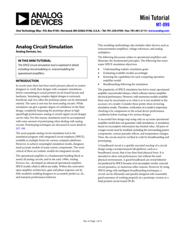
Mini TutorialMT-099One Technology Way P.O. Box 9106 Norwood, MA 02062-9106, U.S.A. Tel: 781.329.4700 Fax: 781.461.3113 www.analog.comThis modeling methodology also includes other devices such asinstrumentation amplifiers, voltage references, and analogmultipliers.Analog Circuit SimulationAnalog Devices, Inc.The following discussion relates to operational amplifiers andillustrates the fundamental principles. The following lists somemajor SPICE simulation objectives:IN THIS MINI TUTORIALThe SPICE circuit simulation tool is explored in detail,including micromodeling vs. macromodeling foroperational amplifiers. INTRODUCTIONIn recent years there has been much pressure placed on systemdesigners to verify their designs with computer simulationsbefore committing to actual printed circuit board layouts andhardware. Simulating complex digital designs is extremelybeneficial, and very often the prototype phase can be eliminatedentirely. The same is not true for most analog circuits. Whilesimulation can give a greater degree of confidence in the finaldesign, completely bypassing the prototype phase in highspeed/high performance analog or mixed-signal circuit designscan be risky. For this reason, simulation must be accompaniedwith some amount of prototyping when dealing with analogcircuits. Prototyping techniques are discussed in more detail inMT-100.The most popular analog circuit simulation tool is thesimulation program with integrated circuit emphasis (SPICE),available in multiple forms for various computer platforms.However, to achieve meaningful simulation results, designersneed accurate models of many system components. The mostcritical of these are realistic models for integrated circuits.The operational amplifier is a fundamental building block innearly all analog circuits, and in the early 1990s, AnalogDevices, Inc., developed an advanced operational amplifierSPICE model, which is still in use today. Within this innovativeopen amplifier architecture, gain and phase response can befully modeled, enabling designers to accurately predict ac, dc,and transient performance behavior. Understanding realistic simulation goalsEvaluating available models accordinglyKnowing the capabilities for each competing operationamplifier modelBreadboarding following the simulationThe popularity of SPICE simulation has led to many operationalamplifier macromodel releases, which software mimics amplifierelectrical performance. However, with numerous models availablethere may be uncertainty as to what is or is not modeled or theaccuracy of a model. Consider these points when reviewingsimulation results. Therefore, verification of a model is important,checking it by comparison to the actual device performanceconditions before trusting it for serious designs.A successful first design step using only an accurate operationalamplifier model does not guarantee valid simulations. A simulationbased on incomplete information has limited value. All parts ofa target circuit must be modeled, including the surrounding passivecomponents, various parasitic effects, and temperature changes.Then, the circuit must be verified in a lab by breadboarding andprototyping.A breadboard circuit is a quickly executed mockup of a circuitdesign using a semipermanent lab platform, such as abreadboard circuit, that is less than final physical form. It isintended to show real performance, but without the totalphysical environment. A good breadboard can reveal behaviornot predicted by SPICE because of an incomplete model, externalcircuit parasitics, or numerous other reasons. However, by usingSPICE along with intelligent breadboarding techniques, acircuit can be efficiently and quickly designed with reasonablygood assurance of working properly on a prototype version or afinal printed circuit board (PCB).Rev. A Page 1 of 12
MT-099Mini TutorialTABLE OF CONTENTSIn This Mini Tutorial. 1Current Feedback Amplifier Models .9Introduction . 1Modeling PC Board Parasitics . 10Revision History . 2Other Design and Simulation Tools . 11Macromodel vs. Micromodel . 3References . 12The SPICE Operational Amplifier Macromodels . 3REVISION HISTORY10/2016—Rev. 0 to Rev. AUpdated Format . UniversalDeleted Figure 1; Renumbered Sequentially. 1Changes to Introduction Section. 1Deleted Figure 2 . 2Added Table 1. 3Changes to Figure 4 and Figure 7 . 7Added Figure 5, Figure 6, and Table 2 . 7Changes to Figure 10, Figure 13, and Figure 16 . 9Added Figure 11, Figure 12, Figure 14, and Figure 15 . 10Added Figure 17 and Figure 18 . 11Changes to Other Design and Simulation Tools Section . 112/2009—Revision 0: Initial VersionRev. A Page 2 of 12
Mini TutorialMT-099MACROMODEL vs. MICROMODELThe distinction between macromodel and micromodel is oftenunclear. A micromodel uses the transistor level and other SPICEmodels of an IC device, with all active and passive parts fullycharacterized according to the manufacturing process. Indifferentiating this type of model from a macromodel, someauthors use the term device level model to describe the resultingoverall operational amplifier model (see the References section).Typically, use a micromodel in the design process of an IC.A macromodel is a less complex way to simulate operationalamplifier performance. Taking into consideration final deviceperformance, it uses ideal native SPICE elements to modelobserved behavior. When developing a macromodel, a realdevice is measured in terms of lab and data sheet performanceand is adjusted to match this behavior. Some aspects ofperformance can be sacrificed in doing this. Table 1 comparesthe major advantages and disadvantages between macromodelsand micromodels.Table 1. Comparison of Macromodels and MicromodelsModelMethodology AdvantagesMacromodel IdealFastelementssimulationmodel device time, easilybehaviormodifiedMicromodel FullyMostcharacterized completetransistor level modelcircuitDisadvantagesMay notmodel allcharacteristicsSlow abilityThere are advantages and disadvantages to both models. Amicromodel can give a complete and accurate model ofoperational amplifier circuit behavior under almost allconditions. But, because of a large number of transistors anddiodes with nonlinear junctions, simulation time is very long.Of course, manufacturers are also reluctant to release suchmodels, since they contain proprietary information. Althoughall transistors can be included, it does not guarantee totalaccuracy, as the transistor models do not cover all operationalregions precisely. Furthermore, with a high node count, SPICEcan have convergence difficulties, causing a failed simulation.This point makes a micromodel virtually useless for multipleamplifier active filters.A carefully developed macromodel can produce both accurateresults and simulation time savings. In more advanced macromodels, transient and ac device performance can be similarlyreplicated. Operational amplifier nonlinear behavior can also beincluded, such as output voltage and current swing limits.However, because these macromodels are still simplifications ofreal devices, all nonlinearities are not modeled. For example, not allSPICE models include common-mode input voltage range or noise.Typically, in model development, parameters are optimizedspecifically for the intended application; for example, ac andtransient response.Including every possible characteristic can lead to cumbersomemacromodels that can have convergence problems. Thus,SPICE macromodels include those operational amplifierbehavior characteristics critical to intended performance fornormal operating conditions, but not necessarily all nonlinearbehavior.THE SPICE OPERATIONAL AMPLIFIERMACROMODELSThe basic SPICE model was developed as an operationalamplifier macromodeling advance and as an improved designtool for more accurate application circuit simulations. Sincebeing introduced in 1990, it has become a standard operationalamplifier macromodel topology, as evidenced by industryadoption of the frequency shaping concepts; refer to AN-840and AN-856.Prior to about 1990, a dominant operational amplifier modelarchitecture was the Boyle model (see the References section).This macromodel, developed in the early 1970s, cannot accuratelymodel higher speed amplifiers. The primary reason for this isthat it has limited frequency shaping ability—only two poles and nozeroes. In contrast, the SPICE model topology has a flexible andopen architecture, allowing virtually unlimited pole and zerofrequency shaping stages to be cascaded. This difference provides amore accurate ac and transient response compared to the moresimplistic Boyle model topology.A SPICE model is comprised of three main stages. The first is acombined input and gain stage that includes transistor modelsappropriate to the device being modeled (for example, NPNbipolar transistor, PNP bipolar transistor, junction gate fieldeffect transistor (JFET), or metal–oxide–semiconductor fieldeffect transistor (MOSFET)).The second stage is the synthetic pole and zero stage, comprisingof ideal SPICE native elements. Depending on the frequencyresponse of the operational amplifier, there can be few to manypole and zero stages. The third stage is an output stage, whichcouples the first two sections to the outside world.Before describing these sections in detail, it is important torealize that many variations upon the following techniques doexist. This is due to not just differences from one operationalamplifier model to another, but also to evolutionary topologydevelopments in operational amplifier hardware, which leads tocorresponding modeling changes. For example, modernoperational amplifiers often include either rail-to-rail outputstages, rail-to-rail input stages, or both. Consequently, morerecent developments in the SPICE models have addressed theseissues, along with corresponding model developments.Furthermore, although the Boyle model and the original SPICEmodels are designed to support voltage feedback operationalamplifier topologies, subsequent additions have added currentfeedback amplifier topologies. Reference 9 describes an SPICEcurrent feedback macromodel which appeared just shortly afterthe voltage feedback model of Reference 3.Rev. A Page 3 of 12
MT-099Mini TutorialThe controlled source, gm1, senses the differential collectorvoltage, VD, from the input stage, converting VD to a proportionalcurrent. The gm1 output current flows into load Resistor R7,producing a single-ended voltage referenced to an internal voltage,EREF. Typically, this voltage is derived as a supply voltage midpointand is used throughout the model.These current feedback macromodels are discussed in moredetail in the following sections.Input and Gain/Pole StagesA basic SPICE voltage feedback operational amplifiermacromodel input stage is shown in Figure 1 and uses what aretypically the only transistors in the entire model. The examplein Figure 1 shows the Q1 to Q2 NPN pair. These are needed toproperly model the differential input stage characteristics of anoperational amplifier. This stage is designed for unity gain bythe proper choice of the Q1 to Q2 operating current and gainsetting resistors R3 to R4 and R5 to R6.By making the gm1 to R7 product equal to the specified gain ofthe operational amplifier, this stage produces the entire openloop gain of the macromodel. This design factor means that allother model stages operate at unity gain, a feature leading tosignificant flexibility in adding and deleting subsequent stages.This approach allows the quick synthesis of the complex accharacteristics typical of high performance, high speed operationalamplifiers. In addition, this stage also provides the dominant poleof the amplifier ac response. The open-loop pole frequency isset by selection of capacitor C3, as noted in the diagram.Although this example uses NPN transistors, the input stage iseasily modified to use PNP bipolars, JFET, or MOSFET devices.The rest of the input stage uses simple SPICE elements such asresistors, capacitors, and controlled sources.The open-loop gain vs. frequency characteristics of the modeledoperational amplifier is provided by the gain stage (see Figure 1). VSR3R4C2– PUT STAGEGAIN UNITYEREFENI–VSOPEN LOOP GAIN/POLE STAGEGAIN gm1 R7Figure 1. Input and Gain/Pole Stages of SPICE MacromodelRev. A Page 4 of 1214826-001IN
Mini TutorialMT-099Frequency Shaping StagesFollowing the gain stage of the macromodel is a variable, butunlimited, number of pole and/or zero stages, which incombination provide frequency response shaping. Typicaltopologies for these stages are as shown in Figure 2. The stagescan be either a single pole, a single zero, or combined pole/zeroor zero/pole stages. All such stages have a dc transfer gain ofunity and a given amplifier type can have all or just a few ofthese stages, as can be require to synthesize the response.The pole or zero frequency is set by the combination of theresistor(s) and capacitor or resistor(s) and inductor. Because aninfinite number of values are possible in SPICE, choice of resistor/capacitor (RC) values is somewhat arbitrary, and a wide rangework. Early SPICE models used relatively RC high values, whilemore recent models employ lower RC values to reduce noise(described in more detail later). In all instances, it is assumedthat each stage provides zero loading to the driving stage. Thestages shown reflect no particular operational amplifier, butexample principles can be found within the OP27 model.Because all of these frequency shaping stages are dc-coupledand have unity gain, any number of the stages can be added ordeleted with no affect on the model low frequency response.Most importantly, the high frequency gain and phase responsecan be tailored to match a real amplifier response. The benefitsof this frequency shaping flexibility are apparent in performancecomparisons of the SPICE model closed-loop pulse responseand stability analysis, versus a more simplistic model. This pointis demonstrated in the Transient Response section.C5R9gm2R8E1C4EREFR10EREFZERO STAGER10 1R9 R10POLE STAGEgm2 R8 1E1 R11R14gm3gm4R13R12C6POLE/ZERO STAGEgm4 R13 1ZERO/POLE STAGEgm3 R11 1Figure 2. The Frequency Shaping Stages Possible Within the SPICE ModelRev. A Page 5 of 1214826-002EREFEREF
MT-099Mini TutorialOutput Stagesthat such an output stage has a voltage gain greater than one.The third point is the relatively high output impedance, whichis high contrasted to traditional emitter follower outputs.A general form of the output stage for the SPICE model, shownin Figure 3, models a number of important operational amplifiercharacteristics. The Thevenin equivalent resistance of RO1 andRO2 mimics the operational amplifier dc open-loop outputimpedance, while the inductor local oscillator (LO) models therise in impedance at high frequencies. A unity-gain characteristicfor the stage is set by the g7 to RO1 and g8 to RO2 products.Additionally, output load current is correctly reflected in thesupply currents. This feature is a significant improvement overthe Boyle model because the power consumption of the loadedcircuit can be analyzed accurately. Furthermore, circuits usingthe operational amplifier supply currents as part of the signalpath can also be correctly simulated. The output stage, shown inFigure 3, is not intended to reflect any particular operationalamplifier, but resembles the AD817.Examples of several modeling approaches to rail-to-rail outputstages are found in the ADI SPICE macromodel library. TheOP295 employs complementary metal-oxide semiconductor(CMOS) devices to realize a rail-to-rail output, while the OP284uses bipolar devices to the same end. The macromodels of theAD8031 and AD823 use synthesis techniques to model rail-torail outputs. The AD8051/AD8052/AD8054, AD8552, andAD623 utilize combinations of selected discrete device modelsand synthesis techniques, to realize rail-to-rail output operationfor both operational amplifier and instrumentation amplifierdevices.In addition to rail-to-rail output operation, many modernoperational amplifiers also feature rail-to-rail input stages. Suchstages essentially duplicate, for example, an NPN-based differentialstage with a complementary PNP stage, both stages operating inparallel. This allows the operational amplifier to provide acommon-mode (CM) range that includes both supply rails. Thisperformance feature can also be accomplished within CMOSoperational amplifiers, using both a P and N type CMOSdifferential pairs. Model examples reflecting rail-to-railinput stages include the OP284, AD8031, and AD8552.With the recent advent of numerous rail-to-rail output stageoperational amplifiers, there are currently customized modeltopologies. This expands the SPICE library to include rail-torail model behavior, matching operational amplifier architecturesusing P and N MOSFET devices, as well as bipolar devices.Characteristically, a rail-to-rail output stage includes severalkey differentiating performance points.The first point is the ability to swing the operational amplifieroutput within a few mV of both supplies. The second point is TPUT IMPEDANCE RO1 RO22 sLOFigure 3. General-Purpose Macromodel Output StageRev. A Page 6 of 1214826-003EREF
Mini TutorialMT-099Transient ResponseNoise ModelThe performance advantage of the multiple pole/zero stages isreadily demonstrated in a transient pulse response test (see Figure 4to Figure 6). These figures compare the OP249 operationalamplifier, the SPICE model, and the Boyle model. It reveals theimproved execution resulting from the unlimited number ofpoles and zeros in this model.An important enhancement to the SPICE model is the ability torealistically model noise performance of an operational amplifierand is easier than analyzing noise by hand. A complete analysis isan involved and tedious task that involves adding all individualnoise contributions from all active devices and all resistors inuse, and referring them to the input.To aid this task, the SPICE model is enhanced to include noisegenerators that accurately mimic the broadband and 1/f noise ofan operational amplifier.1009050mV/DIVConceptually, this involves making an existing model noiselessand then adding discrete noise generators to emulate the targetdevice. As noted earlier, all Analog Devices models are notnecessarily designed for this noise accurate performance.Selected device models are designed for noise, however, whentypical uses include low noise applications.1014826-0040%200ns/DIVThe first step is an exercise in scaling down the model internalimpedances. For example, by reducing the resistances in thepole/zero stages from a base resistance of 1 MΩ to 1 Ω, totalnoise is reduced dramatically, shown in Figure 7 and Table 2.Figure 4. Pulse Response Comparison of an OP249 Follower100LOAD 260pFVOLTAGE (mV)500gm2R9C400.51.0TIME (µs)1.52.0EREF14826-005–100Figure 7. Reducing Pole/Zero Cell Impedances to Low Values to Achieve LowNoise OperationFigure 5. Model Favors the SPICE Model in Terms of Fidelity100Table 2. Parameter Noise ComparisonLOAD 260pFParameterR9gm2C4NoiseVOLTAGE (mV)500.51.0TIME re 6. Model Does Not Favor the Boyle Model in Terms of FidelityUsing the OP249 amplifier, with the output connected to theinverting input and a 260 pF capacitive load, Figure 4 to Figure 6shows the transient analysis plots for a unity gain follower circuit.Noisy1 106 Ω1 10 6159 10 15129 nV/ HzNoiseless1Ω1.0159 10 8129 pV/ HzIn the Noisy column of Table 2, the noise from the pole stagewith a large R9 resistor value is 129 nV/ Hz. But when this resistoris scaled down by a factor of 1 106 to 1 Ω in the Noiseless column,stage noise is 129 pV/ Hz. The transconductance and capacitancevalues are also scaled by the same factor, maintaining the samegain and pole frequency. To make the input stage of the modelnoiseless, it is operated at a high current and with reduced loadresistances, making noise contributions negligible. Extending thesetechniques to the entire model renders it essentially noiseless.This results in ringing, shown in Figure 4. Note that the SPICEmodel accurately predicts the amount of overshoot andfrequency of the damped ringing (see Figure 5). In contrast, theBoyle model (see Figure 6) predicts about half the overshoot andsignificantly less ringing.Rev. A Page 7 of 12
MT-099Mini 826-008RNOISE1EREFFigure 8. A Basic SPICE Noise Generator Formed with Diodes, Resistors,and Controlled SourcesOnce achieving global noise reduction is achieved, addindependent noise sources, one for voltage noise and two forcurrent noise. The basic noise source topology used as seen inFigure 8, and can be set up to produce both voltage and currentnoise outputs.Within SPICE, semiconductor models can generate flicker noise(1/f). The noise generators use diodes, such as DN1, to producethis portion of the noise, modeling the 1/f noise of theoperational amplifier. By properly specifying diode modelparameters and bias voltage VNOISE1, the 1/f noise is tailoredto match the operational amplifier. The noise current from DN1passes through a zero voltage source. Here, VMEAS is used as ameasurement device, combining the 1/f noise from DN1 andthe broadband noise from RNOISE1.RNOISE1 is selected to provide an appropriate broadband noise(see Figure 8). The combined noise current in VMEAS ismonitored by FNOISE (see Figure 8), and appears as a voltageacross RNOISE2. This voltage is injected in series with oneamplifier input via a controlled voltage source, such as EN ofFigure 1. Use either FNOISE or a controlled voltage sourcecoefficient for overall noise voltage scaling.Current noise generation is similar, except the RNOISE2 voltageproducing resistor is not used and two current controlledsources drive the amplifier inputs. With all noise generatorssymmetrical about ground, dc errors are not introduced.Rev. A Page 8 of 12
Mini TutorialMT-09999R1GB1 C1I1V1V39D1 GB213D3CS185R3Q3G16LS1G230VOSR5 IN 32C3–IN972R474Q4EREFCS2I2 C2R2 D4D214V2V45014826-0091Figure 9. Input and Gain Stages of Current Feedback operational amplifier MacromodelThe four bipolar transistor input stage resembles actual currentfeedback amplifiers, with a high impedance noninverting input( IN) and a low impedance inverting input ( IN). In currentfeedback amplifiers, the maximum slew rate is very high,because dynamic slew current is not limited to a differentialpair tail current (voltage feedback operational amplifiers). Incurrent feedback operational amplifier designs, much largeramounts of error current can flow in the inverting input, asdeveloped by the feedback network. Internally, this currentflows in either Q3 or Q4, and charges the C3 compensationcapacitor via current mirrors.The current feedback amplifier input and gain stage is anenhancement to the SPICE model that increases flexibility inmodeling different operational amplifier devices and provides anet increase in design cycle speed.The current mirrors of the SPICE model are actually voltagecontrolled current sources in the G1 and G2 gain stages. Theysense voltage drops across the R1 and R2 input stage resistors,and translate into the C3 charging current. By making the valueof G1 and G2 equal to the R1 to R2 reciprocal, the slew currentsare identical. By clamping the R1 to R2 voltage drops via D1 toV1 and D2 to V2, the maximum current is limited, setting thehighest slew rate. Open loop gain or transresistance of themodel is set by R5 and the open loop pole frequency by C3 toR5 (see Figure 1). The output from across R5 to C3 (Node 12)drives the succeeding frequency shaping stages of the model,and EREF is again an internal reference voltage.Rev. A Page 9 of 1284RF 500ΩRF 1kΩ0–4–81M10MFREQUENCY (Hz)100MFigure 10. Real AD811 Current Feedback Operational Amplifier14826-010As noted previously, a new model topology is developed forcurrent feedback amplifiers to accommodate the unique inputstage structure. The model uses a topology, shown in Figure 9,for the input and gain stages. The remaining model portions(not shown) contain multiple pole/zero stages and the outputstage, and are essentially the same as voltage feedbackamplifiers, described previously in the Input and Gain/PoleStages section.A unique property of current feedback amplifiers is thatbandwidth is a function of the feedback resistor and the internalcompensation capacitor, C3. The lower the feedback resistor,the greater the bandwidth, until a practical lower limit isreached, that is, the value at which the device oscillates. As themodel includes a low impedance inverting input, it accuratelymimics real device behavior as radio frequency (RF) is altered.Figure 10 to Figure 12 compares the SPICE model to the AD811video amplifier. As shown in Figure 10 and Figure 11, the modelaccurately predicts the gain roll-off at the much lower frequencyfor the 1 kΩ feedback resistor as opposed to the 500 Ω resistor.GAIN (dB)CURRENT FEEDBACK AMPLIFIER MODELS
MT-099Mini Tutorial850mV/DIVRF 1kΩGAIN (dB)10090RF ENCY (Hz)1G14826-011Figure 14. Lab Testing Results200Figure 11. Macromodel AD811 Current Feedback Operational AmplifierVOLTAGE (mV)100RF150Ω14826-012RF20–100–200MODELING PC BOARD PARASITICSPCB parasitics can have significant impact on the performanceof a circuit. This is especially true for high speed circuits. A fewpicofarads of capacitance on the input node can determinewhether a circuit is stable or oscillates and must be carefullyconsidered when simulating the circuit to achieve meaningfulresults.To illustrate the impact of PCB parasitics, the simple voltagefollower circuit of Figure 14 is built on a carefully laid out PCBand on a component plug in type of prototype board. Use theAD847 operational amplifier because of the50 MHz bandwidth,making the parasitic effects more critical (smaller values ofcapacitance have a greater effect on results).0100200300TIME (ns)40014826-015Figure 12. AD811 Simulation Circuit500Figure 15. Simulation ResultsHowever, the same circuit built on the plug in prototype boardshows distinctly different results. In general, the prototypeboard shows worse performance due to the relatively high nodalcapacitances around the operational amplifier inputs, degradingthe square wave response to severe ringing, much less than thefull capability of the device (see Figure 16 and Figure 17).AD84765pF50ns/DIV14826-013 50Ω14826-017845ΩFigure 16. Without Low Parasitics, Lab Testing Results Show ConvergenceWith A Poorly Damped ResponseFigure 13. Voltage FollowerAs a result, this circuit executed on a carefully laid out PCB hasa clean response with minor overshoot and ringing (see Figure 14).The SPICE model results also closely agree with the real device,showing a corresponding simulation (see Figure 15).Rev. A Page 10 of 12
Mini TutorialMT-099200Parasitic PCB elements are not the only area that can causedifferences between the simulation and the breadboard. Acircuit can exhibit nonlinear behavior during power-up thatcauses a device to lock up. Or, a device can oscillate due toinsufficient power supply decoupling or lead inductance.VOLTAGE (mV)1000SPICE circuits do not need bypassing, but real world onesalways need bypassing. It is impossible to anticipate all normalor abnormal operating conditions to which an amplifier mightbe subjected.–2000100200300TIME (ns)40050014826-018–100Figure 17. Without Low Parasitics, Parallel Simulation Show ConvergenceWith A Poorly Damped ResponseThe voltage follower circuit, Figure 18, shows the additionalcapacitances as inherent to the prototype board. With this testcircuit and corresponding analysis, there is, initially, noagreement between the poor lab test and the parallel SPICE test.However, when the relevant PCB parasitic capacitances areincluded in the SPICE file, then the simulation results do agreewith the real circuit, as noted in the right picture.2pF 845Ω 8pF50Ω 8pF65pF14826-016AD847It is always important to prototype circuits and thoroughlycheck them in the lab. Careful forethought in these stages ofdesign minimizes any unknown problems from showing upwhen the final PCBs are manufactured.OTHER DESIGN AND SIMULATION TOOLSAnalog Devices has a large number of useful design toolslocated at the Design Center on the Analog Devices website.ADIsimPE, which is powered by SIMetrix/SIMPLIS, is a circuitsimulation suite optimized for the design and development ofanalog and mixed signal circuits. The SIMetrix mode is ideal forthe simulation of general nonswitching circuits. It provides fullPSpice compatibility for use with industry-standard SPICEmodels. The SIMPLIS mode simulates the operation ofswitching circuits with vastly improved robustness, speed,
Mini Tutorial MT-099 OneTechnologyWay P.O.Box9106 Norwood,MA 02062-9106,U.S.A. Tel:781.329.4700 Fax:781.461.3113 www.analog.com Rev. A Page 1 of 12 Analog Circuit Simulation . Analog Devices, Inc. IN THIS MINI T UTORIAL illustr The SPICE circuit simulation tool is explored in detail, including micromodeling vs. macromodeling for