Transcription
College of Saint BenedictSt. Joseph, MNGreenhouse Gas Emissions InventoryReport1992-2008Report Issue Date: July 2008Project Team:Marnie McInnisMelissa Gearman
1. Summary and Overview2. Inventory Processa. Clean Air Cool Planet Carbon Calculatorb. Methodologyc. Limitationsd. Data sources and contacts3. Inventory Results4. Transportation Inventorya. Introductionb. Resultsc. Data sources and contact information5. Energy Emissions Inventorya. Introductionb. Resultsc. Data sources and contact information6. Landscape Emissions Inventorya. Introductionb. Resultsc. Data sources and contact information7. Solid Waste Emissions Inventorya. Introductionb. Resultsc. Data sources and contact information8. Refrigerants Emissions Inventorya. Introductionb. Resultsc. Data sources and contact information9. Offsetsa. Introductionb. Resultsc. Data sources and contact information2
1. SummaryThis report reviews the College of Saint Benedict’s green house gas emissions using theClean Air Cool Planet Carbon Calculator. This tool covers greenhouse emissions coveredby the Kyoto Protocol, Including Carbon Dioxide (CO2), Methane (CH4), nitrous oxide (N20),hydrofluorocarbons (HFC), perfluorocarbons (PFCs) and sulphur hexafluoride (SF6).The emissions report covers fiscal years 1992-2008.The inventory process was completed in accordance with the American College &University Presidents Climate Commitment. Completing an emissions inventory is aprimary step in defining the amount of emissions The College of Saint Benedict emits. Byfinding emissions data, The College of Saint Benedict is able to track their greenhousegas emissions and come closer to ultimately achieving carbon neutrality.2. Inventory Processa. Clean Air-Cool Planet Campus Carbon CalculatorClean Air-Cool Planet (CA-CP) is a nonprofit organization that provides a Microsoft Excelspreadsheet to calculate greenhouse gas emissions for participating corporations,communities, and campuses. It is currently in use by over 200 schools in North America.The spreadsheet allows for input of information into separate categories includinginstitutional data, transportation, solid waste, and refrigeration. As data is input into thespreadsheet, CA-CP estimates total greenhouse gas emissions. The spreadsheetprovides graphs and charts to illustrate trends in greenhouse gas emissions. Tocomplete this inventory, version 5.0 was used.b. MethodologyThe Campus Carbon Calculator specifies seven categories of data in order to make itscalculations. These categories include: Institutional Data, Purchased Electricity, Steamand Chilled Water, On Campus Stationary Sources of Energy, Transportation,Agriculture, Solid Waste, Refrigeration, and Carbon Offsets. Each category is brokeninto detailed subcategories. Not all categories are relevant to each organization.c. LimitationsWhile conducting the inventory, data regarding transportation was difficult to gather.While completing the calculation of non-commuter vehicle miles traveled by students,faculty, and staff a survey was used to estimate miles traveled. This model haslimitations since survey data is often unreliable and inaccurate. In the future, theinstitution may want to complete a more comprehensive survey for a more accuratemodel of non-commuter vehicle miles traveled.
Data was collected for air miles traveled based on corporate travel card charges. Thereported data does not include travel expenses for reimbursement forms. In the future,the College is planning on requesting miles traveled on reimbursement forms for moreaccurate data.d. Data Sources and ContactsInstitutional Data:Budget:Anne ObermanControllerCSB Business OfficeExt. 5999aoberman@csbsju.eduPopulation:Data Source: Full-Time Students: CSB/SJU institutional data fact f/FactBook2007.pdfPhysical Size:Jim SchumannInterim Chief Physical PlantCSB Mary Commons 127Ext. 5211jschumann@csbsju.eduData Source: lities/academic.htmPurchased Electricity:Terry LosoPower Plant Director1411 Co Rd 134St Joseph, MN 56374ext. 5109tloso@csbsju.eduTransportationGasoline Fleet:Dorothy GanglPurchasing CoordinatorCSB Main 230Ext. 5353dgangl@csbsju.eduDiesel Fleet:Mike JuntunenTransportation Director4
CSB Maintenence BuildingExt. 5789mjuntunen@csbsju.eduAir Travel:Faculty/Staff Business:Anne Oberman:ControllerCSB Business OfficeExt. 5999aoberman@csbsju.eduCommuter:Jean LavigneProfessorSJU NewSc 114Ext. 3994jlavigne@csbsju.eduData Source: Faculty/Staff Business: GIS coordinates and SurveyAgriculture:Fertilizer Application:Chris BrakeGrounds SupervisorCSB Maintanence BuildingExt. 5976cbrake@csbsju.eduSolid Waste:Jim SchumannInterim Chief Physical PlantCSB Mary Commons 127Ext. 5211jschumann@csbsju.eduRefrigeration and other chemicals:Ganard OrionziDirector of Environmental Health and SafetyCSB Main and PENGL 201Ext. 5277 (CSB) and Ext. 3267 (SJU)gorionzi@csbsju.edu5
3. Inventory ResultsThe objective for the inventory was to see previous emissions data for comparison inthe future. There is not consistent data dating back to the 1992 fiscal year; certain datawas only available for different years. Specifically, solid waste, fertilizer application, andstudent/faculty and staff commuter data was only available for the 2008 fiscal year.Annually, the College of Saint Benedict emits an average of 15212.81 metric tonsgreen house gases in carbon dioxide equivalence.In 2008, the College of Saint Benedict emitted 21823.11 metric tons of greenhouse gases in carbon dioxide equivalence. Figure one below details the sourcesof emissions in 2008.2008 Emissions OverviewSolid Waste7%Transport Total30%Figure e 2 below shows emissions by scope since the 1992 fiscal year. “Emissions byScope” refers to the origin of the emissions. Scope one emissions refer to all emissionsof greenhouse gasses from sources that are owned or controlled by The College of SaintBenedict. This includes emissions generated such as fuel used by campus vehicles andHydrofluorocarbon leakage from refrigeration and/or air conditioning units on campus.Scope two emissions include emissions by power plants released producing electricityfor the institution. Scope three emissions encompass all other indirect emissions. Thisincludes emissions that result from institutional action but are from sources neitherowned nor controlled by the institution. The sharp rise of scope three emissions in 2008is due to the data that was only available for that fiscal year. At The College of SaintBenedict, Scope 2 emissions are the single largest contributor to green house gas
emissions. Thus, electricity produced to for the institution contributes most green housegas emissions.Emissions By ScopeTotal Emissions (Metric Tonnes eCO2)25,01020,01015,010Scope 3 Emissions10,010Scope 2 EmissionsScope 1 08Figure 2.Figure 3 below illustrates the metric tons of CO2 equivalent per full time students. Thisgraph has approximately the same shape as that of the graph of total emissions.Metric Tons eCO2 / Student Full Time EquivalentTotal Emissions per Student(Metric Tons eCO2 / Student FTE)12108642019921994199619982000Figure 3.72002200420062008
Figure 4 below shows the trend between the addition of building space and totalemissions. With additional space, total building efficiency has not increased. However,total emissions reached a low in 2006. This could be attributed to CSB doing lightingretrofitting to replace inefficient lighting with more efficient devices. In 2008, the totalemissions per square foot of building space was 17.8.Kilogram (kg) eCO2 / Square Foot Building SpaceTotal Emissions per square foot(kg eCO2 / ft 2 ure 4.Figure 5 shows the square footage of CSB from 1990-2008. The size of CSB steadilyincreased from 1990-1996 and leveled of until present. With the addition of the GoreckiDining and Conference Center in 2007, the square footage increased. As the amount ofsquare footage the campus has increases, the rise in carbon emissions can be attributedto the increased building space.Square Feet of Building Space at CSB from 1990-20081,300,000Building Space (Square 000600,000500,00019901992199419961998Figure 5.820002002200420062008
4. Transportationa. IntroductionTransportation fueled by the burning of gasoline, diesel, and jet fuel contributeconsiderably to carbon dioxide emissions. The Clean Air Cool Planet calculator showedthat transportation is a minor contributor of green house gas emissions For CSB.Categories that were inventoried were:CSB Vehicle fleetLink Bus ServiceAir travel by faculty and staffDaily commute by students, faculty, and staffb. ResultsThe CSB vehicle fleet is used for moving equipment around campus, maintenance ofgrounds, and other college related needs.The link bus service, providing transportation from CSB to St. John’s University, includesdiesel used by college owned buses and contracted Trobec’s Busing Service. BecauseThe Link is a combined department between CSB and SJU, the amount total amount ofdiesel used by the Link was divided between the two campuses. The Link emits a yearlyaverage of 185.3 Metric Tons of carbon dioxide.The graph below shows the amount of diesel used by the Link from 2005-2008. As seen,there is a drop in the amount of diesel used in 2007. CSB stopped contracting as manybuses from Trobec’s Busing Service in 2007, which led to a decrease of mileage by about5,202. The values used in the carbon calculator were half of what is seen in the graphbecause the amount of diesel used by the Link was split equally between CSB and SJU.Total Diesel Used by the Link50,00048,000Diesel 032,00030,000200520062007Figure 6.92008
The following graph shows the amount of students transported by the Link from 20052008. The amount of passengers on the Link has risen steadily since 2005. In 2008, theLink offered more bussing service, including busing service over breaks.Total students transported by the LinkNumber of Students 00006500006000002005200620072008Figure 7.The following chart shows the emissions given off by the link in carbon dioxide values.The chart follows the came basic trend as the amount of diesel used by the Link.Carbon Emissions (Metric Tons)Carbon Emissons by the Link200195190185180175170165160200520062007Figure 8.102008
For air travel information, data was collected for air miles traveled based on corporatetravel card charges. Travel expenses one reimbursement forms are not included in thereported data. A formula was used to derive the amount of miles flown based on travelexpenses, .25 1 mile traveled. In the future, the College is planning on requesting milestraveled on reimbursement forms for more accurate data. Student air travel miles werecalculated for the number of miles students traveled on study abroad trips. Alsoincluded in the 2008 student air miles is the number of miles traveled in schoolsponsored alternative spring break trips. Data for these air miles were only available forthe 2007-2008 fiscal year.In order to figure out how far faculty and staff were commuting a mapping softwareprogram named Arcmap was used. A map of Minnesota zip codes and cities inMinnesota was used to point on the map roughly halfway between St. John’s and St.Ben’s. The program then calculated the center of each zip code polygon. Manually usingthe programs measuring tool, the centered to each zip code to the point between St.John’s and St. Ben’s was measured. Then, a round trip distance was approximated.Using the number of zip codes that were obtained, information on a per person basiswas obtained. However, the number of zip codes that were used did not match up withthe number of faculty and staff employed on campus. Thus, division was used to applythe data to the current numbers of faculty and staff. Through this, the distance of howfar each faculty member was traveling per day was found. It was assumed each facultymember was driving alone and the majority of the faculty worked most weekdaysthroughout the year.To find how often and how far students are driving survey results were used. Thesurveys had information on how often students were driving per week, how often theywere alone when driving, how often they were with someone else when driving,approximations of how far they are driving, and an estimated fuel economy for theirvehicle. Using this data, approximations were found based on how far each student wasdriving per week on average. This also provided information on how often studentswere alone or carpooling and gave an average fuel economy for the campus. Having allthe numbers per student allowed the information to be applied to the entire campusthrough simple multiplication. The number of miles traveled by each student, each daywas put into the carbon calculator. In order to determine the number of days per yeareach student is driving, the number of days and weekends that students are on campuswas counted.c. Data sources and contact informationContact:Mike JuntunenTransportation DirectorCSB Maintenence BuildingExt. 5789mjuntunen@csbsju.edu11
Faculty/Staff Business Air TravelAnne Oberman:ControllerCSB Business OfficeExt. 5999aoberman@csbsju.edu5. Energy Emissions Inventorya. IntroductionIt is expected that energy emissions will contribute over 90% of emissions by CSB.Energy emissions are split up into on-campus stationary sources, off-campus electricityproduction, and off-campus steam production. On-campus stationary sources apply tofuel purchased by CSB other than gasoline or diesel fuel used in vehicles. CSB is heatedusing a combination of oil and natural gas. Off-campus electricity production refers tohow much electricity was purchased by CSB. This includes electricity used for lighting,computers, cooking, and air conditioning. Greenhouse gases associated with energyinclude carbon dioxide and nitrous oxide during the combustion of fossil fuels andmethane from natural gas.The monastery is included in the total amount of energy used by CSB. The data for thecollege and the monastery is able to be separated dating back to 2001. However,separating subsequent to 2001 would cause an error in the long term trend of energyuse.b. ResultsFigure 9 shows the overall total emissions at CSB. The numbers are relatively consistentfrom 1992 to 2006. The large spike between fiscal years 2007 and 2008 results from theadded data from refrigerants and other chemicals and solid waste and more completetransportation data.12
Total Emissions at the College of Saint BenedictTotal Emissions (Metric Tonnes eCO2)25,000Refrigerants and otherChemicalsSolid Waste20,000Transportation15,000On-campus Stationary10,000Purchased 008Figure 9.The graph below displays the amount of purchased electricity consumed by CSB. Thepurchased electricity peaks during 1999-2000 at 10,258,000 kWh. In 2000, CSB installedthe Central Chilled Water Plant and discontinued the use of individual units for all thebuildings that used more electricity than the more efficient chiller plant. Also, starting in2000, CSB has done lighting retrofitting to replace inefficient lighting with more efficientdevices.Purchased Electricity Consumed at CSB (kWh)Purchased ,000,0002,000,00001992Figure 10.1994199619982000Year132002200420062008
Figure 11 below displays the amount of electricity consumed per student at CSB. Asnoted above, the amount of electricity peaks at 1996 and again in 1999. The amount ofelectricity consumed per student remains considerably even from 2001-2008.kWh electricity consumed per student at CSB6000Electricity 200420062008YearFigure 11.Carbon (Metric Tons)Figure 12 displays the amount of carbon emitted per student from purchased electricity.This graph follows the same trend as the purchased electricity consumed at CSB, withrises in the graph due to the chilled water plant being installed in 2000.54.543.532.521.510.50Total Carbon from purchased Electricity Per Student (MetricTons)1992Figure 12.1994199619982000Year142002200420062008
Figure 13 below shows the temperature trends from 1990-2008 in St. Cloud, MN. Thegraph below shows the number of heating degree days per year (blue) in comparison tothe average number of total degree days since 1990. In 2006 the number of heatingdegree days was lower than the number in the surrounding years. Fewer heating degreedays means it would take less energy to heat buildings during that year. Trends intemperature can provide an explanation for variation in the amount of energy used.Total Heating Degree Days (65 Degree Balance Point) St. Cloud, MNNumber of Heating Degree 19961998Figure 13.20002002200420062008YearThe following graph displays the temperature trends from 1992-2008 and the averagenatural gas use in (MMBtu) consumed at CSB. As seen, the natural gas consumption andtemperature follow the same general trend.Average Heating days compared to Natural Gas consumption at CSB120000900800100000700Axis 9941996199820002002YearFi gure 14.15200420062008Gas (MMBTU)Average Heating Days
The following graphs below illustrate the amount of natural gas and electricity beconsumed by CSB and the estimated cost projections. As seen, the cost is expected torise steadily. By 2020 CSB will be consuming 12,700,174 and spending 1,964,360 onelectricity. For natural gas, by 2020 CSB will be consuming 113,881 MMBtu of naturalgas and spending 595,935.Electricity Projections fromFY2005 Average Building Efficiencies andInstitutional Growth Rate 1990-200514000000 2,500,00012000000Electric Demand (kWh) 2,000,00010000000 1,500,00080000006000000 1,000,000DemandCost4000000 500,00020000000 02002200420062008201020122014201620182020Figure 15.Natural Gas Projections fromFY2005 Average Building Efficiencies andInstitutional Growth Rate 1990-2005Natural Gas Demand (MMBtu)250,000 1,000,000 900,000200,000 800,000 700,000150,000 600,000 500,000100,000 400,000 300,00050,000 200,000 100,000- 02002200420062008201020122014Figure 16.16201620182020DemandCost
c. Data Sources and Contact InformationTerry LosoPower Plant Director1411 Co Rd 134St Joseph, MN 56374ext. 5109tloso@csbsju.edu6. Agriculture and Landscapea. IntroductionAgriculture and landscaping are major contributors of methane (CH4) and nitrous oxide(N2O) both of which are major greenhouse gases. Methane emissions commonly comefrom animals, especially dairy cows, in the form of bacteria in the gut of the cow and thedecomposition of manure. Nitrous oxide is a gas given off by fertilizers after application.Synthetic fertilizers are labeled with three numbers representing their chemical makeup. The numbers represent the percent nitrogen (N), phosphorus (P), and potassium(K); so a fertilizer labeled 15-15-10 is 15 percent nitrogen.b. ResultsThe College of Saint Benedict does not have any livestock or agricultural practices andtherefore does not need to worry about those emissions. Instead, this sectionconcentrates on the fertilizer application on campus grounds. Records of pastapplications were not kept so only the fiscal year 2007 amounts were reported. Thegrounds around the president’s house, the athletic fields, and the mall between theHaehn Campus Center and the Benedicta Arts Center, a total of 25 acres, used 5 tons of30-0-15 fertilizer. The grounds around the Main, Library, and around the Benedicta ArtsCenter, a total of 15 acres, used 3 tons of 10-0-10 fertilizer. This calculated to a total of8 tons of fertilizer with an average of 23 percent nitrogen.The following graph shows the major contributors of nitrous oxide emissions. Even withonly a single year of data it is visible that fertilizer can contribute greatly to the overallnitrous oxide emissions total. Purchased electricity is the only other emission sourcethat contributes as greatly as landscaping. The spike in the graph is due to the fact thatmore data is available for fiscal year 2007 and 2008.17
Total Nitrous Oxide Emissions500Nitrous Oxide Emissions (kg campus 62008Figure 17c.Data sources and contact informationA soil test was conducted by the University of Minnesota soil testing laboratory todetermine the optimal ratio of nutrients for different areas of the campus. CampusGrounds at CSB then uses this information when deciding fertilizes to use on campus.Contact:Chris BrakeCSB Grounds SupervisorCSB Maintenance Buildingcbrake@csbsju.edu7. Solid Wastea. IntroductionSolid waste is disposed in one of two methods: incineration or landfills. Incineratedwaste releases greenhouse gases when it is burned while waste that goes to landfillsrelease methane as it decomposes. After the waste is picked up it is disposed of in oneof several different ways ranging from simple incineration to a landfill that collects themethane emissions for electric generation. This calculator uses emissions from an“average” composition of waste.b. Results18
The College of Saint Benedict does not have good records of the amount of solid wastethat is generated on campus. Only an estimate of one year, fiscal year 2008, was able tobe calculated based on the size of the waste container and frequency of pickup. Acalculation table was then used to calculate a rough estimate of the amount of solidwaste produced. CSB generated around 1,529 tons of sold waste last year.Solid waste is the only major contributor of methane (CH4) on campus. CSB waste issent to a landfill where CH4 collection does not take place. It released close to 68,000kg of CH4 into the atmosphere.c. Data Sources and contact informationTo calculate an estimate of the amount of solid waste generated, a waste capacitycalculation found on the city of Durham, North Carolina solid waste web page1. Againthis is a rough estimate. In the future better record keeping will result in more reliableinformation.8. Refrigeration and other chemicalsa. IntroductionRefrigerants such as hydrofluorocarbons (HFCs) and perfluorocarbons (PFCs) are used asalternatives to chlorofluorocarbons (CFCs). Under the terms of the Montreal Protocoland the U.S. Clean Air Act, CFCs and other known harmful refrigerants are being phasedout and being replaced by HFCs and PFCs. However, HFCs and PFCs are known to bestrong greenhouse gases as well. Because CFCs are being phased out they do not needto be included in the inventory but all other refrigerants should be included.b. ResultsThe College of Saint Benedict does not keep a record of how much refrigeration or othersuch chemicals it has on campus. This is because of the fact that no major leaks havebeen reported and because of the size of the school. St. Ben’s is a small school andtherefore does not have as big or as many appliances that would use refrigerants as alarge university would. The amount of refrigeration and other chemicals on campus is avery small amount.c. Data Sources and contact informationContact:Ganard OrionziDirector of Environmental Health and SafetyMain Building G40 (CSB), PENGL 201 (SJU)1SWM Capacity Calculation Information, apacitycalculation.pdf (December 2005)19
gorionzi@csbsju.edu9. Offsetsa. IntroductionMany institutions decide to offset some greenhouse gas emissions. Certain institutionfunded activities such as air travel are unavoidable and will inevitably produce somegreenhouse gas emissions. These emissions can be offset in a number of ways, but onethe most common is the purchase of Tradable Renewable Energy Certificates (TREC),also known as “Green Tags”. These certificates are created when electricity is createdby some form of renewable energy, wind, solar, or small scale hydroelectric. Each creditrepresents one megawatt-hour of electricity was created by renewable energy. Pricesfor RECs range from 5 to 90. The energy created does not have to be on the samegrid as the institution and therefore cannot just be subtracted from total electricemissions. Instead it must be added separately. Other offsets an institution maypartake in include protecting a forest that acts as a carbon sink or composting.b. ResultsThe College of Saint Benedict does not purchase any offsets to mitigate any of itsgreenhouse gas emissions.20
The spreadsheet allows for input of information into separate categories including institutional data, transportation, solid waste, and refrigeration. As data is input into the spreadsheet, CA-CP estimates total greenhouse gas emissions. The spreadsheet provides graphs and charts to illustrate trends in greenhouse gas emissions. To