WIXLIB

310.91 - p-valueAs mentioned, a major benefit of the bootstrap isthat any evaluation metric can be used to computeδ(x).3 We run the bootstrap using several metrics:F1-measure for constituency parsing, unlabeled dependency accuracy for dependency parsing, alignment error rate (AER) for word alignment, ROUGEscore (Lin, 2004) for summarization, and BLEUscore for machine translation.4 We report all metrics as percentages.0.8Different research groupsSame research group0.70.6Experiments0.5Our first goal is to explore the relationship between metric gain, δ(x), and statistical significance,p-value(x), for a range of NLP tasks. In order to sayanything meaningful, we will need to see both δ(x)and p-value(x) for many pairs of systems.3.1Natural ComparisonsIdeally, for a given task and test set we could obtainoutputs from all systems that have been evaluatedin published work. For each pair of these systemswe could run a comparison and compute both δ(x)and p-value(x). While obtaining such data is notgenerally feasible, for several tasks there are public competitions to which systems are submitted bymany researchers. Some of these competitions makesystem outputs publicly available. We obtained system outputs from the TAC 2008 workshop on automatic summarization (Dang and Owczarzak, 2008),the CoNLL 2007 shared task on dependency parsing(Nivre et al., 2007), and the WMT 2010 workshopon machine translation (Callison-Burch et al., 2010).For cases where the metric linearly decomposes over sentences,the mean of δ(x(i) ) is δ(x). By the central limit theorem, thedistribution will be symmetric for large test sets; for small testsets it may not.3Note that the bootstrap procedure given only approximatesthe true significance level, with multiple sources of approximation error. One is the error introduced from using a finite number of bootstrap samples. Another comes from the assumptionthat the bootstrap samples reflect the underlying population distribution. A third is the assumption that the mean bootstrap gainis the test gain (which could be further corrected for if the metricis sufficiently ill-behaved).4To save time, we can compute δ(x) for each bootstrap sample without having to rerun the evaluation metric. For our metrics, sufficient statistics can be recorded for each sentence andthen sampled along with the sentences when constructing eachx(i) (e.g. size of gold, size of guess, and number correct are sufficient for F1). This makes the bootstrap very fast in practice.99700.51ROUGE1.52Figure 2:TAC 2008 Summarization: Confidence vs.ROUGE improvement on TAC 2008 test set for comparisonsbetween all pairs of the 58 participating systems at TAC 2008.Comparisons between systems entered by the same researchgroup and comparisons between systems entered by differentresearch groups are shown separately.3.1.1TAC 2008 SummarizationIn our first experiment, we use the outputs of the58 systems that participated in the TAC 2008 workshop on automatic summarization. For each possible pairing, we compute δ(x) and p-value(x) on thenon-update portion of the TAC 2008 test set (we order each pair so that the gain, δ(x), is always positive).5 For this task, test instances correspond todocument collections. The test set consists of 48document collections, each with a human producedsummary. Figure 2 plots the ROUGE gain against1 p-value, which we refer to as confidence. Eachpoint on the graph corresponds to an individual pairof systems.As expected, larger gains in ROUGE correspondto higher confidences. The curved shape of the plotis interesting. It suggests that relatively quickly wereach ROUGE gains for which, in practice, significance tests will most likely be positive. We mightexpect that systems whose outputs are highly correlated will achieve higher confidence at lower metric gains. To test this hypothesis, in Figure 2 we5In order to run bootstraps between all pairs of systemsquickly, we reuse a random sample counts matrix between bootstrap runs. As a result, we no longer need to perform quadratically many corpus resamplings. The speed-up from this approach is enormous, but one undesirable effect is that the bootstrap estimation noise between different runs is correlated. As aremedy, we set b so large that the correlated noise is not visiblein plots.

11 - p-value0.90.8Different research groupsSame research group0.70.60.500.511.522.5Unlabeled Acc.33.54Figure 3: CoNLL 2007 Dependency parsing: Confidence vs.unlabeled dependency accuracy improvement on the ChineseCoNLL 2007 test set for comparisons between all pairs of the21 participating systems in CoNLL 2007 shared task. Comparisons between systems entered by the same research groupand comparisons between systems entered by different researchgroups are shown separately.separately show the comparisons between systemsentered by the same research group and comparisons between systems entered by different researchgroups, with the expectation that systems entered bythe same group are likely to have more correlatedoutputs. Many of the comparisons between systemssubmitted by the same group are offset from themain curve. It appears that they do achieve higherconfidences at lower metric gains.Given the huge number of system comparisons inFigure 2, one obvious question to ask is whetherwe can take the results of all these statistical significance tests and estimate a ROUGE improvementthreshold that predicts when future statistical significance tests will probably be significant at thep-value(x) 0.05 level. For example, let’s say wetake all the comparisons with p-value between 0.04and 0.06 (47 comparisons in all in this case). Eachof these comparisons has an associated metric gain,and by taking, say, the 95th percentile of these metric gains, we get a potentially useful threshold. Inthis case, the computed threshold is 1.10 ROUGE.What does this threshold mean? Well, based onthe way we computed it, it suggests that if somebodyreports a ROUGE increase of around 1.10 on the exact same test set, there is a pretty good chance that astatistical significance test would show significanceat the p-value(x) 0.05 level. After all, 95% of998the borderline significant differences that we’ve already seen showed an increase of even less than 1.10ROUGE. If we’re evaluating past work, or are insome other setting where system outputs just aren’tavailable, the threshold could guide our interpretation of reports containing only summary scores.That being said, it is important that we don’t overinterpret the meaning of the 1.10 ROUGE threshold.We have already seen that pairs of systems submitted by the same research group and by different research groups follow different trends, and we willsoon see more evidence demonstrating the importance of system correlation in determining the relationship between metric gain and confidence. Additionally, in Section 4, we will see that properties ofthe test corpus have a large effect on the trend. Thereare many factors are at work, and so, of course, metric gain alone will not fully determine the outcomeof a paired significance test.3.1.2CoNLL 2007 Dependency ParsingNext, we run an experiment for dependency parsing. We use the outputs of the 21 systems that participated in the CoNLL 2007 shared task on dependency parsing. In Figure 3, we plot, for all pairs,the gain in unlabeled dependency accuracy againstconfidence on the CoNLL 2007 Chinese test set,which consists of 690 sentences and parses. Weagain separate comparisons between systems submitted by the same research group and those submitted by different groups, although for this task therewere fewer cases of multiple submission. The results resemble the plot for summarization; we againsee a curve-shaped trend, and comparisons betweensystems from the same group (few that they are)achieve higher confidences at lower metric gains.3.1.3WMT 2010 Machine TranslationOur final task for which system outputs are publicly available is machine translation. We run an experiment using the outputs of the 31 systems participating in WMT 2010 on the system combinationportion of the German-English WMT 2010 news testset, which consists of 2,034 German sentences andEnglish translations. We again run comparisons forpairs of participating systems. We plot gain in testBLEU score against confidence in Figure 4. In thisexperiment there is an additional class of compar-

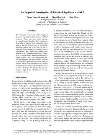
11 - p-value0.90.8Different research groupsSame research groupSystem combination0.70.60.500.20.40.60.81BLEUFigure 4: WMT 2010 Machine translation: Confidence vs.BLEU improvement on the system combination portion of theGerman-English WMT 2010 news test set for comparisons between pairs of the 31 participating systems at WMT 2010.Comparisons between systems entered by the same researchgroup, comparisons between systems entered by different research groups, and comparisons between system combinationentries are shown separately.isons that are likely to have specially correlated systems: 13 of the submitted systems are system combinations, and each take into account the same setof proposed translations. We separate comparisonsinto three sets: comparisons between non-combinedsystems entered by different research groups, comparisons between non-combined systems entered bythe same research group, and comparisons betweensystem-combinations.We see the same curve-shaped trend we saw forsummarization and dependency parsing. Different group comparisons, same group comparisons,and system combination comparisons form distinctcurves. This indicates, again, that comparisons between systems that are expected to be specially correlated achieve high confidence at lower metric gainlevels.3.2Synthetic ComparisonsSo far, we have seen a clear empirical effect, but, because of the limited availability of system outputs,we have only considered a few tasks. We now propose a simple method that captures the shape of theeffect, and use it to extend our analysis.3.2.1Training Set ResamplingAnother way of obtaining many different systems’ outputs is to obtain implementations of a999handful of systems, and then vary some aspect ofthe training procedure in order to produce many different systems from each implementation. Koehn(2004) uses this sort of amplification; he uses a single machine translation implementation, and thentrains it from different source languages. We takea slightly different approach. For each task we picksome fixed training set. Then we generate resampledtraining sets by sampling sentences with replacement from the original. In this way, we can generate as many new training sets as we like, each ofwhich is similar to the original, but with some variation. For each base implementation, we train a newsystem on each resampled training set. This resultsin slightly tweaked trained systems, and is intendedto very roughly approximate the variance introducedby incremental system changes during research. Wevalidate this method by comparing plots obtained bythe synthetic approach with plots obtained from natural comparisons.We expect that each new system will be different, but that systems originating from the same basemodel will be highly correlated. This provides a useful division of comparisons: those between systemsbuilt with the same model, and those between systems built with different models. The first class canbe used to approximate comparisons of systems thatare expected to be specially correlated, and the latterfor comparisons of systems that are not.3.2.2Dependency ParsingWe use three base models for dependency parsing:MST parser (McDonald et al., 2005), Maltparser(Nivre et al., 2006), and the ensemble parser of Surdeanu and Manning (2010). We use the CoNLL2007 Chinese training set, which consists of 57Ksentences. We resample 5 training sets of 57K sentences, 10 training sets of 28K sentences, and 10training sets of 14K sentences. Together, this yieldsa total of 75 system outputs on the CoNLL 2007Chinese test set, 25 systems for each base modeltype. The score ranges of all the base models overlap. This ensures that for each pair of model typeswe will be able to see comparisons where the metricgains are small. The results of the pairwise comparisons of all 75 system outputs are shown in Figure5, along with the results of the CoNLL 2007 sharedtask system comparisons from Figure 3.

10.90.90.81 - p-value1 - p-value1Different model typesSame model typeCoNLL 2007 comparisons0.70.60.8Different model typesSame model typeWMT 2010 comparisons0.70.60.50.500.511.522.5Unlabeled Acc.33.5400.20.40.60.81BLEUFigure 5: Dependency parsing: Confidence vs. unlabeled de-Figure 6: Machine translation: Confidence vs. BLEU im-pendency accuracy improvement on the Chinese CoNLL 2007test set for comparisons between all pairs of systems generated by using resampled training sets to train either MST parser,Maltparser, or the ensemble parser. Comparisons between systems generated using the same base model type and comparisons between systems generated using different base modeltypes are shown separately. The CoNLL 2007 shared task comparisons from Figure 3 are also shown.provement on the system combination portion of the GermanEnglish WMT 2010 news test set for comparisons between allpairs of systems generated by using resampled training sets totrain either Moses or Joshua. Comparisons between systemsgenerated using the same base model type and comparisons between systems generated using different base model types areshown separately. The WMT 2010 workshop comparisons fromFigure 4 are also shown.The overlay of the natural comparisons suggeststhat the synthetic approach reasonably models therelationship between metric gain and confidence.Additionally, the different model type and samemodel type comparisons exhibit the behavior wewould expect, matching the curves corresponding tocomparisons between specially correlated systemsand standard comparisons respectively.labeled accuracy by 1.3, it is useful to be able toquickly estimate that the improvement is probablysignificant. This still isn’t the full story; we willsoon see that properties of the test set also play amajor role. But first, we carry our analysis to several more tasks.Since our synthetic approach yields a large number of system outputs, we can use the proceduredescribed in Section 3.1.1 to compute the threshold above which the metric gain is probably significant. For comparisons between systems of the samemodel type, the threshold is 1.20 unlabeled dependency accuracy. For comparisons between systemsof different model types, the threshold is 1.51 unlabeled dependency accuracy. These results indicate that the similarity of the systems being compared is an important factor. As mentioned, rulesof-thumb derived from such thresholds cannot beapplied blindly, but, in special cases where two systems are known to be correlated, the former threshold should be preferred over the latter. For example,during development most comparisons are made between incremental variants of the same system. Ifadding a feature to a supervised parser increases un10003.2.3 Machine TranslationOur two base models for machine translationare Moses (Koehn et al., 2007) and Joshua (Li etal., 2009). We use 1.4M sentence pairs from theGerman-English portion of the WMT-provided Europarl (Koehn, 2005) and news commentary corporaas the original training set. We resample 75 trainingsets, 20 of 1.4M sentence pairs, 29 of 350K sentencepairs, and 26 of 88K sentence pairs. This yields atotal of 150 system outputs on the system combination portion of the German-English WMT 2010news test set. The results of the pairwise comparisons of all 150 system outputs are shown in Figure6, along with the results of the WMT 2010 workshopsystem comparisons from Figure 4.The natural comparisons from the WMT 2010workshop align well with the comparisons betweensynthetically varied models. Again, the differentmodel type and same model type comparisons formdistinct curves. For comparisons between systems

10.90.91 - p-value1 - p-value10.8Different model typesSame model type0.70.60.8Different model typesSame model type0.70.60.50.500.51AER1.52Figure 7: Word alignment: Confidence vs. AER improvement on the Hansard test set for comparisons between all pairsof systems generated by using resampled training sets to traineither the ITG aligner, the joint HMM aligner, or GIZA .Comparisons between systems generated using the same basemodel type and comparisons between systems generated usingdifferent base model types are shown separately.of the same model type the computed p-value 0.05 threshold is 0.28 BLEU. For comparisons between systems of different model types the thresholdis 0.37 BLEU.3.2.4 Word AlignmentNow that we have validated our simple model ofsystem variation on two tasks, we go on to generate plots for tasks that do not have competitionswith publicly available system outputs. The firsttask is English-French word alignment, where weuse three base models: the ITG aligner of Haghighiet al. (2009), the joint HMM aligner of Liang et al.(2006), and GIZA (Och and Ney, 2003). The lasttwo aligners are unsupervised, while the first is supervised. We train the unsupervised word alignersusing the 1.1M sentence pair Hansard training corpus, resampling 20 training sets of the same size.6Following Haghighi et al. (2009), we train the supervised ITG aligner using the first 337 sentence pairsof the hand-aligned Hansard test set; again, we resample 20 training sets of the same size as the original data. We test on the remaining 100 hand-alignedsentence pairs from the Hansard test set.Unlike previous plots, the points correspondingto comparisons between systems with different base6GIZA failed to produce reasonable output when trainedwith some of these training sets, so there are fewer than 20GIZA systems in our comparisons.100100.51F11.52Figure 8: Constituency parsing: Confidence vs. F1 improvement on section 23 of the WSJ corpus for comparisons betweenall pairs of systems generated by using resampled training setsto train either the Berkeley parser, the Stanford parser, or theCollins parser. Comparisons between systems generated using the same base model type and comparisons between systems generated using different base model types are shown separately.model types form two distinct curves. It turns outthat the upper curve consists only of comparisonsbetween ITG and HMM aligners. This is likely dueto the fact that the ITG aligner uses posteriors fromthe HMM aligner for some of its features, so thetwo models are particularly correlated. Overall, thespread of this plot is larger than previous ones. Thismay be due to the small size of the test set, or possibly some additional variance introduced by unsupervised training. For comparisons between systems ofthe same model type the p-value 0.05 thresholdis 0.50 AER. For comparisons between systems ofdifferent model types the threshold is 1.12 AER.3.2.5Constituency ParsingFinally, before we move on to further types ofanalysis, we run an experiment for the task of constituency parsing. We use three base models: theBerkeley parser (Petrov et al., 2006), the Stanfordparser (Klein and Manning, 2003), and Dan Bikel’simplementation (Bikel, 2004) of the Collins parser(Collins, 1999). We use sections 2-21 of the WSJcorpus (Marcus et al., 1993), which consists of 38Ksentences and parses, as a training set. We resample10 training sets of size 38K, 10 of size 19K, and 10of size 9K, and use these to train systems. We teston section 23. The results are shown in Figure 8.For comparisons between systems of the same

model type, the p-value 0.05 threshold is 0.47F1. For comparisons between systems of differentmodel types the threshold is 0.57 F1.4.1Varying the SizeFigure 9 plots comparisons for machine translationon variously sized initial segments of the WMT2010 news test set. Similarly, Figure 10 plots comparisons for constituency parsing on initial segmentsof the Brown corpus. As might be expected, thesize of the test corpus has a large effect. For bothmachine translation and constituency parsing, thelarger the corpus size, the lower the threshold forp-value 0.05 and the smaller the spread of theplot. At one extreme, the entire Brown corpus,which consists of approximately 24K sentences, hasa threshold of 0.22 F1, while at the other extreme,the first 100 sentences of the Brown corpus have athreshold of 3.00 F1. Notice that we see diminishingreturns as we increase the size of the test set. Thisphenomenon follows the general shape of the central limit theorem, which predicts that variances ofobserved metric gains will shrink according to thesquare root of the test size. Even using the entireBrown corpus as a test set there is a small rangewhere the result of a paired significance test was notcompletely determined by metric gain.It is interesting to note that for a fixed test size,the domain has only a small effect on the shape ofthe curve. Figure 11 plots comparisons for a fixedtest size, but with various test corpora.10021 - p-valueFor five tasks, we have seen a trend relating metric gain and confidence, and we have seen that thelevel of correlation between the systems being compared affects the location of the curve. Next, welook at how the size and domain of the test set playa role, and, finally, how significance level predictsperformance on held

An Empirical Investigation of Statistical Signicance in NLP Taylor Berg-Kirkpatrick David Burkett Dan Klein Computer Science Division University of California at Berkeley ftberg, dburkett, klein g@cs.berkeley.edu . tems. Public competitions, such as the well-known CoNLLsharedtasks, provideonenaturalwaytoob-tain a variety of system outputs on .