Transcription
Thermo-PileA software for the geotechnical design of energy pilesUSER’S MANUALLaboratory of Soil MechanicsSwiss Federal Institute of Technology Lausannehttp://lms.epfl.chv1.0
Thermo-Pile: User’s Manualpage 1Copyright by EPFL LMSAll rights reserved. No part of this document may be reproduced or otherwise used inany form without express written permission from EPFL.Soil Mechanics Laboratory (LMS)Prof. L. LalouiSwiss Federal Institute of Technology Lausanne (EPFL)Station 18, 1015 Lausanne, SwitzerlandCopyright Swiss Federal Institute of Technology Lausanne (EPFL), Laboratory of Soil Mechanics (LMS)
Thermo-Pile: User’s Manualpage 2TABLE OF CONTENT1 INTRODUCTION . 31.2 GOAL OF THERMO-PILE . 31.3 THE CONTENT OF THE TECHNICAL MANUAL. 31.4 THE CONTENT OF THIS MANUAL . 32 STARTING THERMO-PILE . 42.1 INSTALLING THERMO-PILE . 42.2 FIRST START . 43 GRAPHICAL USER INTERFACE (GUI) . 44 READING AND WRITING FILES . 54.1 READING AND WRITING PROJECTS FROM MAIN MENU . 54.2 LOADING RESULTS . 74.3 SPECIFYING THERMAL LOADING BY READING A FILE. 85 UNITS SYSTEM AND SIGN CONVENTIONS . 86 RUNNING A PROJECT – SPECIFYING GEOMETRIES AND PROPERTIES . 86.1 SOIL GEOMETRY AND PHYSICAL PROPERTIES (MODEL SOILPROPERTIES) . 96.2 PILE PROPERTIES (MODEL PILE PROPERTIES). 106.3 PILE-SOIL AND PILE-STRUCTURE INTERACTIONS (MODEL INTERFACEPROPERTIES) . 116.4 MECHANICAL AND THERMAL LOADINGS (MODEL LOADING). 137. VISUALIZING RESULTS (GRAPHS) . 148. CLOSING THERMO-PILE (PROJECT EXIT) . 149. SHORTCUTS FOR USING THERMO-PILE WITH KEYBOARD . 1410. EXEMPLES: SOME CASE STUDIES. 1510.1 EPFL CASE STUDY . 1510.2 PARAMETRIC STUDIES . 2411 FAQ . 2712. KNOWN ISSUES . 2812.1 INCREMENT SIZE CRITERIA . 2812.2 ABOUT ACCURACY AND PILE DISCRETIZATION . 2812.3 SOFTWARE’S LIMTATIONS . 2813 THERMO-PILE MESSAGES . 2913.1 ERROR MESSAGES . 2913.2 OTHER MESSAGES . 29REFERENCES . 30Copyright Swiss Federal Institute of Technology Lausanne (EPFL), Laboratory of Soil Mechanics (LMS)
Thermo-Pile: User’s Manualpage 31 INTRODUCTION1.1 IMPORTANT NOTICE*Safety factors are not included in the calculation process.*Only one pile with circular section is considered.*Tensile mechanical solicitation and bending moments are not considered.*Negative friction is not considered.1.2 GOAL OF THERMO-PILEThe principal goal of the software Thermo-Pile is to determine the extra stresses anddisplacements that come from the temperature variations (thermal solicitations) in aheat exchanger foundation pile. Classical pile calculation (verification of the bearingcapacity and settlement calculation) can also be performed, by setting thetemperatures constant.1.3 THE CONTENT OF THE TECHNICAL MANUALThe manual named Thermo-Pile Documentation Theory explains in details themethod used in Thermo-Pile and gives the necessary background to understand it. Itis based on the paper: Knellwolf C., Peron H. and Laloui L. “Geotechnical analysis ofheat exchanger piles”. Journal of Geotechnical and Geoenvironmental Engineering,doi: 10.1061 / (ASCE) GT.1943-5606.0000513, 2011.1.4 THE CONTENT OF THIS MANUALThe main sections of this manual are:Section 2: How to run Thermo-Pile on any machine.Section 3: Overview of the Graphical User Interface of Thermo-Pile.Section 4: Writing/loading file module of Thermo-Pile.Section 5: Unit system and conventions used in Thermo-Pile.Section 6: Available tools to design your project.Section 7: Graphics menu to visualize results within Thermo-Pile.Section 8: How to exit / close Thermo-Pile.Section 9: Keyboard shortcuts of the menu.Section 10: Some case studies with Thermo-Pile.Section 11: FAQ.Section 12: Known issues.Copyright Swiss Federal Institute of Technology Lausanne (EPFL), Laboratory of Soil Mechanics (LMS)
Thermo-Pile: User’s Manualpage 42 STARTING THERMO-PILE2.1 INSTALLING THERMO-PILEIf not yet installed, Thermo-Pile requires the Java Runtime Environment (JRE 1.6 atleast) which can be downloaded at java.com.To install Thermo-Pile on a machine, launch the Thermo-Pile Setup and follow theinstructions of the wizard. The specified folder during the installation will be the folderwhere all the projects will be saved.Once Thermo-Pile is installed on a machine, the user needs to activate it on first startbefore using it (see Section 2.2).2.2 FIRST STARTTo launch the software, just double click on the Thermo-Pile.exe file.At the first start of Thermo-Pile on a machine, you will have to follow different steps inorder to activate your Thermo-Pile version:1. Communicate the red characters (see figure 0) and the name of your companyby email to lms@epfl.ch with the object “Thermo-Pile Activation”.2. Copy and paste the activation key provided by your supplier in the Activationkey box and click Activate.3. Restart the Thermo-Pile application.Fig 0. Activation window of Thermo-Pile.3 GRAPHICAL USER INTERFACE (GUI)The Thermo-Pile GUI is divided into four main panels:-The main menu panel (1), from where all the menus are accessible;The project name (2), corresponding to the currently running project;The results panel (3) where a summary of the results is available;The graphics panel (4), where results profiles are plotted.Copyright Swiss Federal Institute of Technology Lausanne (EPFL), Laboratory of Soil Mechanics (LMS)
Thermo-Pile: User’s Manualpage 51234Fig.1. Main window with 1) Main menu, 2)Project name, 3) Summary of results and 4)Plot space.4 READING AND WRITING FILESSaved files (e.g. projects) from Thermo-Pile, which are parameters files (E.txt) orresults (Res.txt), are located in the same folder as the software (e.g. the application).In order to load a file (E.txt), make sure it is located in the same folder as theapplication you are using.4.1 READING AND WRITING PROJECTS FROM MAIN MENUIn the main menu, reading and writing a project is available in Project Save projector Load Project. Before writing or loading a project, make sure you gave theright prefix (panel 2 in Fig. 1).The prefix represents the name of your project. Then, parameters from your projectwill be saved in a file named YourProjectNameE.txt.The E.txt exported files have the following template:Table 1: Description of the rows of a E.txt file#1234# ofColumns1NBRLAYNBRLAYNBRLAYRow NameCommentNBRLAYDPTLAYNBINCRFRIANGINTNumber of LayersLower depth of a layer on the z axisNumber of increments per layerInternal friction angleCopyright Swiss Federal Institute of Technology Lausanne (EPFL), Laboratory of Soil Mechanics (LMS)
Thermo-Pile: User’s 351nomFICHTEMPpage 6CohesionSpecific weight of the soilInterface friction angleMenard pressuremeter elastic modulusUltimate shear stressUltimate bearing capacity at the baseGroundwater tablePile lengthPile diameterYoung’s modulus of the pileThermal expansion coefficient of the pileLinear spring value for the pile structureInteractionTemperature variation from manual entryMechanical solicitationTheory used to assess the bearing capacityCorrection factor for Lang&Huder theoryKind of enter the thermal loadingTheory for the t-z curvesSlope 1 for branch 1 of the ts-z curveSlope 2 for branch 2 of the ts-z curveSlope 3 for branch 3 of the ts-z curveFraction of qs at the end of branch 1 (ts-zcurve)Fraction of qs at the end of branch 2 (ts-zcurve)Fraction of qs at the end of branch 3 (ts-zcurve)Slope 1 for branch 1 of the ts-z curveSlope 2 for branch 2 of the ts-z curveSlope 3 for branch 3 of the ts-z curveFraction of qs at the end of branch 1 (ts-zcurve)Fraction of qs at the end of branch 2 (ts-zcurve)Fraction of qs at the end of branch 3 (ts-zcurve)ASCII code of the name of the temperaturefileCopyright Swiss Federal Institute of Technology Lausanne (EPFL), Laboratory of Soil Mechanics (LMS)
Thermo-Pile: User’s Manualpage 74.2 LOADING RESULTSOnce the calculation is done, Thermo-Pile automatically generates a file containingthe results and named YourProjectNameRes.txt with the template given in Tables 2and 3. This file is automatically loaded into the software so you can directly visualizethe results thanks to the Graphs menu. You can also reload results from an olderproject by specifying the right prefix and loading the results: Graphs Load Resultsfile. Once again, make sure the results file is in the same folder as the application.Table 2: Description of the rows of a Res.txt fileRow 1Names of the columnsRows 2 to Line NumEle 1Values of the resultsTable 3: Description of the columns if a Res.txt file#Column Name1Depth Blocked15AxialFreeStrainPosition on the z axis for results of columns 2 to10Axial stress after mechanical loadingAxial stress due to thermal loadingAxial stress after thermal loading ( AxialstressMec AxialStressTherm)Axial displacement after mechanical loadingAxial displacement due to thermal loadingAxial displacement after thermal loading ( AxialDisplMec AxialDisplTherm)Mobilised bearing forces after mechanical loadingMobilised bearing forces after thermal loadingUltimate bearing capacityPosition on the z axis for results of columns 12 to10Axial strain after mechanical loadingAxial strain due to thermal loadingPart of the free strain, which is blocked byexternal constraints (springs)Free axial strain th, f ressTotDegreeOffFreedomqsUltimeMenardElasticShear stress mobilised by mechanical loadingShear stress due to thermal loadingShear stress mobilised after thermal loadingDegree of freedomUltimate shear stress valueMenard pressuremeter elastic modulusSignificanceCopyright Swiss Federal Institute of Technology Lausanne (EPFL), Laboratory of Soil Mechanics (LMS)
Thermo-Pile: User’s Manual22ModulusdiffTemperaturepage 8Applied change in temperature4.3 SPECIFYING THERMAL LOADING BY READING A FILEYou can specify the thermal field if it is not homogeneous along the pile. To do so,one must create a .txt file, which has the template as defined in Tables 4 and 5, in thesame directory as your project and load it when specifying the thermal loading on thepile. Just select Model Loading, “Read from txt file” in the Thermal Loading dropmenu and give the right file name.Table 4: Description of the rows of a temperature fileRows 1 to the endData#12Table 5: Description of the columns of a temperature fileColumn NameSignificancePosition on the z axisChange in temperatureThe columns are delimited by a blank space. The number of rows and the position onthe z axis do not need to correspond to the number of pile elements. Thetemperature change assigned to a pile element is that of the closest position from thetemperature file. The comparisons are done with absolute values, so the sign doesnot influence the distances between pile elements and temperature file positions.5 UNITS SYSTEM AND SIGN CONVENTIONSThermo-Pile uses the unit system with seconds, meters and kilograms for the inputparameters and for the results. It cannot be changed. Each parameter unit is given inthe GUI.Upwards displacements and tensile stresses are taken as positive.6 RUNNING A PROJECT – SPECIFYING GEOMETRIES ANDPROPERTIESIn Thermo-Pile, a project consists in specifying a soil (geometry and physicalproperties), a pile (geometry and physical properties), the pile-structure and pile-soilinteractions (parameters and curves) and the pile loading (mechanical and thermalloadings). Those parameters are set in the Model menu.Copyright Swiss Federal Institute of Technology Lausanne (EPFL), Laboratory of Soil Mechanics (LMS)
Thermo-Pile: User’s Manualpage 96.1 SOIL GEOMETRY AND PHYSICAL PROPERTIES (MODEL SOILPROPERTIES)Fig. 2: Soil properties panel.The General panel represents the geometry of the soil. The Number of layers will beuseful to specify different layers with different physical properties. Lower bound oflayers represents the depth at which each layer ends, the origin being the surface.Numbers of increments represents the needed number of elements. A value has tobe specified for each layer. This parameter is important for the result accuracy (seeSection 12.2).The corresponding configuration of the Fig 2 is:SurfaceLayer 110mLayer 215mGroundwater table and Soil Characteristics are available when the Ultimate bearingcapacity method is different from Manual (see Section 6.3 and Table 6).Copyright Swiss Federal Institute of Technology Lausanne (EPFL), Laboratory of Soil Mechanics (LMS)
Thermo-Pile: User’s Manualpage r of layer (n)Lower bound of layers (m)Number of incrementsGroundwater table (m)Internal friction angle ( )Cohesion (kPa)Specific weight of soil (kN m-3)Interface friction angle ( LangTable 6: Soil properties, overview of the theories and their parameters6.2 PILE PROPERTIES (MODEL PILE PROPERTIES)Fig. 3: Pile properties panel.Length and Diameter are the geometric characteristics of the pile (only one cylindricalpile is considered). Young modulus and Thermal expansion coefficient are the pilephysical properties. Chi (Lang&Huder) is a parameter available when the methodLang&Huder: granular soils is enabled for computing the Ultimate Bearing Capacity(see Section 6.3).Copyright Swiss Federal Institute of Technology Lausanne (EPFL), Laboratory of Soil Mechanics (LMS)
Thermo-Pile: User’s Manualpage 116.3 PILE-SOIL AND PILE-STRUCTURE INTERACTIONS (MODEL INTERFACEPROPERTIES)Fig. 4: Interface properties panel.The interactions between the pile and the supported structure, as well as betweenthe pile and the soil are modeled by equivalent springs. In this window the springproperties are defined (see also the technical manual).The spring which models the interaction between the pile head and the supportedstructure (building) is linear elastic. The spring constant is defined by Linear springvalue (see Fig. 4). It is important to underline that even if the mechanical loading isnull, this stiffness is taken into account into the thermal effects calculation. Thus, tomodel free pile head, both mechanical loading and linear spring constant must be setto 0.Ultimate shear stress qs and ultimate bearing capacity at the pile base qb can becalculated using DTU analytic, DTU empiric or Lang&Huder or they can be enteredmanually (Manual). If a theory is chosen, the soil characteristics (see Fig. 4) must bedefined.Copyright Swiss Federal Institute of Technology Lausanne (EPFL), Laboratory of Soil Mechanics (LMS)
Thermo-Pile: User’s Manualpage 12Manual-DTUempiric1nDTUanalyticValue for qs (kPa)Value for qb (kPa)HuderParameter#valuesto enterLangTable 7: Pile – soil interface Properties, ultimate bearing capacity--XXIn the soil – pile interaction, the soil – pile shaft interaction (index s) and the soil pilebase interaction (index b) are distinguished. The springs model the interactionbetween the soil and the pile, and have an elasto-plastic behaviour. The curvesdescribing the spring behaviour are called ts-z and tb-z curves; their shape aredefined by linear branches and a plateau value. t stands for the mobilised shearstress and z for the displacement. One can choose between predefined t-z curves,according to Frank and Zhao for cohesive or granular soils, and user defined t-zcurves (Manual). The theory of Frank and Zhao is based on the Menardpressuremeter elastic modulus and must be entered for each layer. The manual entryallows defining a curve with 3 linear branches and a plateau value. The branches aredefined by their slope K and a shear stress t. (see Fig. 5).The ts,i (resp. tb,i) values aredefined by a fraction of qs (resp. qb).ManualMenard pressuremetermodulus (kPa)Ks1 (kPa m-1)Frank &ZhaocohesivesoilsFrank &Zhaogranular soilsParameter# values toenterTable 8: Pile – soil interface t-z curves1XX-n--XCopyright Swiss Federal Institute of Technology Lausanne (EPFL), Laboratory of Soil Mechanics (LMS)
Thermo-Pile: User’s ManualKs2 (kPa-1)Ks3 (kPa-1)ts1 (kPa)ts2 (kPa)ts3 (kPa)Kb1 (kPa-1)Kb2 (kPa-1)Kb3 (kPa-1)tb1 (kPa)tb2 (kPa)tb3 (kPa)page 13nnnnn111111--XXXXXXXXXXX6.4 MECHANICAL AND THERMAL LOADINGS (MODEL LOADING)Fig. 6: Loading panelMechanical loading represents the building weight. Since no negative friction is takeninto account, the mechanical loading magnitude taken into account is the absolutevalue of the input value and it is oriented downwards. This is the reason whyspecifying a positive or a negative value will not change the results. The thermalloading is relative and can be either a constant value or specified with a .txt file (seeSection 4.3).Copyright Swiss Federal Institute of Technology Lausanne (EPFL), Laboratory of Soil Mechanics (LMS)
Thermo-Pile: User’s Manualpage 147. VISUALIZING RESULTS (GRAPHS)Once the calculation is completed, Thermo-Pile saves a Res.txt file in the samefolder as the project file. This file can then be used to postprocess the results andcreate figures (see Tables 2 and 3). To visualize the results within Thermo-Pile, usethe Graphs menu. Several results versus depth can be displayed.8. CLOSING THERMO-PILE (PROJECT EXIT)Thermo-Pile can be closed thanks to the usual red cross icon on the top right cornerof the window. Nevertheless, it is recommended to close it with the commands in theProject menu Project Save Project and Exit in order to save all changes in yourproject. If you want to quit without saving, use Project Close.9. SHORTCUTS FOR USING THERMO-PILE WITH KEYBOARDTable 9: Menu shortcutsMenuShortcutAlt AAboutAlt GGraphsAlt HHelpAlt M ModelAlt PProjectCopyright Swiss Federal Institute of Technology Lausanne (EPFL), Laboratory of Soil Mechanics (LMS)
Thermo-Pile: User’s Manualpage 1510. EXEMPLES: SOME CASE STUDIES10.1 EPFL CASE STUDY10.1.1 DATAThe example chosen is a full scale in situ test carried out at the EPFL in Lausanne ona heat exchanger pile (see Laloui et al., 2003 and 2006). The heat exchanger pile,which was part of a pile raft supporting a four storey building (Bâtiment Polyvalent,« BP », 100 m in length and 30 m in width) built in 1998-1999 in EPFL Lausanne,was equipped on all its length with load cells, extensometers (both fiber optic andvibrating-wire) and temperature sensors (Laloui et al. 2003, 2006). This pile wassubjected to a thermal load, generated by a heat carrying fluid circulating inpolyethylene pipes embedded in the concrete pile. The pile tested was located at theside of the building. The drilled pile diameter was 88 cm on average, and its lengthwas 25.8 m. Pile integrity tests revealed a slightly marked bulge in the bottom part ofthe pile. The Young modulus of the pile was estimated from laboratory tests andcross-hole ultrasonic transmission tests, yielding the value Epile 29.2 GPa atambient temperature. The coefficient of thermal expansion of the pile was estimatedto be α 1 x 10⁻⁵ C-1.Figure 7 shows the location of the in situ test. The pile geometry and its propertiesare summarized in Table 10.Table 10: Pile characteristicsLength (m)25.8Diameter (m)0.88Young Modulus (kPa)2.82*107Thermal expansion coefficient ( C-1) 10-5A schematic foundation soil profile is presented in Figure 8 (there are five differentsoil layers). The parameters corresponding to the layers and their properties, namelythe lower depth, the bearing capacity at the pile base qb (layer D only), the ultimateshear frictions qs and the rigidity of the soil-pile shaft interaction Ks and soil pile baseinteraction Kb are given in Table11.The soil pile interaction is elasto-plastic, with one linear slope (Ks respectively Kb)starting from zero and ending in a plateau value (qs respectively qb).Copyright Swiss Federal Institute of Technology Lausanne (EPFL), Laboratory of Soil Mechanics (LMS)
Thermo-Pile: User’s Manualpage 1630 m S1202N100 mS1201Pieu-testS1205S1209BP BMBM: bâtiment de microtechniqueBP: bâtiment polyvalentAI: bâtiment d'architectureS1200campagne de sondage 1997Pieu-testAIS1208S1207a)b)Fig. 7 a) Schematic view of the test side b) Aerial view of the EPFLcampusCopyright Swiss Federal Institute of Technology Lausanne (EPFL), Laboratory of Soil Mechanics (LMS)
Thermo-Pile: User’s Manualpage 17Fig. 8 Geological situation of the EPFLpile (Laloui et al. 2003)LayerDepth (m)qs (kPa)qb (kPa)Ks (MPa m-1)Kb(MPa m-1)Table 11: Soil pile interaction .818.2121.4D25.830011000121.4-667.7The pile head building interface spring constant is K 2 GPa/m. The building weightrepresents a solicitation of 1000 kN for the pile. The profile of the thermal solicitationis given in Table 12.Table 12: Profile of change in temperatureDepth (m)ΔT ( C)2.55.512.521.525.817.117.317.117.315.9Copyright Swiss Federal Institute of Technology Lausanne (EPFL), Laboratory of Soil Mechanics (LMS)
Thermo-Pile: User’s Manualpage 1810.1.2 PROCEDURETo open the application, double click on the Thermo-Pile.exe file, then enter theProject’s name (e.g. Example EPFL) in the text field “Project” as shown in Figure 9.Fig.9 Thermo-Pile; Main window10.1.2.1 DEFINITION OF THE MODEL AND SOILD PROPERTIESTo define the increments and to enter the soil properties click in the main menu on: Model Soil PropertiesThere are 5 soil layers with the following number of increments: 11 for layer 1, 20 forlayer 2, 32 for layer 3, 6 for layer 4 and 2 for layer 5.The parameters of the n different layers should be sorted by increasing layer number(e.g. value for the layer 1 up to the value for the layer n) separated with a blankspace in the corresponding text field. Figure 10 shows the completed window “SoilProperties”. To save the values and close the window, click on the OK button.Each text field should contain data for each layer (even if they are disabled). Byclicking on Enter after entering the number of layers, all fields are automatically set tothe correct amount of zeroes which indicates the number of parameters that one hasto specify.Copyright Swiss Federal Institute of Technology Lausanne (EPFL), Laboratory of Soil Mechanics (LMS)
Thermo-Pile: User’s Manualpage 19Fig. 10 Thermo-Pile; Window Soil Properties(Model Soil Properties)Remark:By default, in the Interface Properties window, the option for the assessment of thebearing capacity is set to “Manual”. This means that the parameters for theGroundwater table and the Soil Characteristics are not used for calculation and thusdisabled. To enable them, one has to select a given theory instead of the manualentry option.10.1.2.2 DEFINITION OF THE PILE PROPERTIESAll pile characteristics are constant, so only one value per parameter has to bedefined in the Pile Properties window (Figure 11) Model Soil PropertiesFig. 11 Thermo-Pile; Window PileProperties (Model Pile Properties)Copyright Swiss Federal Institute of Technology Lausanne (EPFL), Laboratory of Soil Mechanics (LMS)
Thermo-Pile: User’s Manualpage 20To save the values and close the window click on the OK button.10.1.2.3 DEFINITION OF THE INTERFACE PROPERTIESThe interfaces are defined in the Interface Properties window: Model Interface PropertiesThe Pile – Structure Interaction Linear spring constant is set to 1'500'000 kPa/m.Since the bearing capacities qs and qb are already known, they can be enteredmanually (the option Manual must then be chosen). The t-z curves for the pile shaftsoil interaction are also entered manually. The Manual option must therefore bechosen. The shape of the t-z curve is explained in Figure 5. In the present example, itconsists of only one linear branch with the slope K s (respectively Kb), followed by aplateau value. Consequently, all Ks slopes of the t-z curves are set equal (Ks1 Ks2 Ks3). The values ts1 and ts2 can be chosen arbitrary between 0 and 1, ts3 has to be setequal to 1 to introduce the plateau. The same procedure is followed to define the t-zcurves for the soil pile base reaction. The complete soil pile interface configuration isshown in Figure 12.Fig.12Thermo-Pile;Window Interface Properties(Model InterfaceProperties)To save the values and close the window click on the OK button.Copyright Swiss Federal Institute of Technology Lausanne (EPFL), Laboratory of Soil Mechanics (LMS)
Thermo-Pile: User’s Manualpage 21Notes:1. If the bearing stresses qb and shear stress qs are assessed by using one ofthe options “Lang&Huder: granular soil”, “DTU analytic: granular soil” or “DTUempiric: granular soil”, the groundwater table and the soil characteristics in Model Soil Interface have to be defined.2. If the t-z curves are not defined manually but by the options “Frank&Zhaogranular soils” or “Frank&Zhao cohesive soils” the text field corresponding tothe Menard pressuremeter elastic modulus for each layer has to be filled in.10.1.2.4 DEFINITION OF LOADSThe mechanical and thermal loads are defined in: Model LoadingThe mechanical loading corresponds to the solicitation of the pile induced by thebuilding weight. According to the sign convention gravity forces are negative.There are two possibilities to enter the thermal loading:1 ) Choose the manual option and put the average value from the givenchanges in temperature into the corresponding text field.2) Create a text file containing the given changes of temperature as showed inFigure 13, with the depths in column 1 and the corresponding temperatures incolumn 2. The two columns are separated by a blank space. The name of the text filecan be chosen arbitrary; here it’s called “thermal Loading”.Fig. 13 Notepad; txt file containingthe thermal loading, column 1: depth,column 2: thermal loadingThen select the option “Read from txt file” and enter the name of the txt field inthe corresponding text field, as shown in Figure 14.Copyright Swiss Federal Institute of Technology Lausanne (EPFL), Laboratory of Soil Mechanics (LMS)
Thermo-Pile: User’s ManualFig. 14Thermo-Pile;Loading (Model Loading)page 22window10.1.2.5 WRITING OF THE E.TXT FILEIn order to save the Model parameters, they must be written in a separate txt file. Todo so, click on: Project Save ProjectNow, a .txt file with the name Example EPFLE.txt should appear in the directory inwhich the Thermo-Pile executable file is stored.10.1.2.6 RUNNING THE CALCULATIONTo run the calculation click on Project Run ProjectFirst the software reads the E.txt file. With the gained information it computes thecalculation and writes the results in a second text file with the ending Res.txt. In ourcase, the file containing the results is named Example EPFLRes.txt.Once the calculation is completed, the message “the calculation has successfullycompleted” appears in the main window.Remark: because the software takes the information from the E.txt file and notdirectly from the text fields in the Model windows, it is important to write theinformation right after modifying parameters. For this reason the Run option isdisabled when the parameters are changed, it becomes enabled only after writing theE.txt file.Copyright Swiss Federal Institute of Technology Lausanne (EPFL), Laboratory of Soil Mechanics (LMS)
Thermo-Pile: User’s Manualpage 2310.1.2.7 PLOTTING GRAPHSTo get the graph, the results are first uploaded form the Res.txt file. To do so, clickon: Graphs Load ResultsTo plot a specific a graph, click on his name. For example, to plot the graph Axialstress versus
Thermo-Pile A software for the geotechnical design of energy piles USER'S MANUAL . Journal of Geotechnical and Geoenvironmental Engineering, doi: 10.1061 / (ASCE) GT.1943-5606.0000513, 2011. . Available tools to design your project. Section 7: Graphics menu to visualize results within Thermo-Pile.


![Pile Foundation Design[1] - ITD](/img/29/pilefoundationdesign.jpg)