Transcription
Linear Models and Conjoint Analysiswith Nonlinear Spline TransformationsWarren F. KuhfeldMark GarrattAbstractMany common data analysis models are based on the general linear univariate model, including linearregression, analysis of variance, and conjoint analysis. This chapter discusses the general linear modelin a framework that allows nonlinear transformations of the variables. We show how to evaluate theeffect of each transformation. Applications to marketing research are presented. Why Use Nonlinear Transformations?In marketing research, as in other areas of data analysis, relationships among variables are not alwayslinear. Consider the problem of modeling product purchasing as a function of product price. Purchasingmay decrease as price increases. For consumers who consider price to be an indication of quality,purchasing may increase as price increases but then start decreasing as the price gets too high. Thenumber of purchases may be a discontinuous function of price with jumps at “round numbers” suchas even dollar amounts. In any case, it is likely that purchasing behavior is not a linear function ofprice. Marketing researchers who model purchasing as a linear function of price may miss valuablenonlinear information in their data. A transformation regression model can be used to investigate thenonlinearities. The data analyst is not required to specify the form of the nonlinear function; the datasuggest the function.The primary purpose of this chapter is to suggest the use of linear regression models with nonlinear transformations of the variables—transformation regression models. It is common in marketingresearch to model nonlinearities by fitting a quadratic polynomial model. Polynomial models oftenhave collinearity problems, but that can be overcome with orthogonal polynomials. The problem thatpolynomials cannot overcome is the fact that polynomial curves are rigid; they do not do a good jobof locally fitting the data. Piecewise polynomials or splines are generalizations of polynomials thatprovide more flexibility than ordinary polynomials. This chapter is a revision of a paper that was presented to the American Marketing Association, Advanced ResearchTechniques Forum, June 14–17, 1992, Lake Tahoe, Nevada. The authors are: Warren F. Kuhfeld, Manager, MultivariateModels R&D, SAS Institute Inc., Cary NC 27513-2414. Mark Garratt was with Conway Milliken & Associates, whenthis paper was presented and is now with In4mation Insights. Copies of this chapter (MR-2010J), sample code, and all ofthe macros are available on the Web e marketresearch.html.All plots in this chapter are produced using ODS Graphics. For help, please contact SAS Technical Support. See page 25for more information.1213
1214MR-2010J — Linear Models and Conjoint Analysis with Nonlinear Spline TransformationsBackground and HistoryThe foundation for our work can be found mostly in the psychometric literature. Some relevantreferences include: Kruskal & Shepard (1974); Young, de Leeuw, & Takane (1976); de Leeuw, Young,& Takane (1976); Perreault & Young (1980); Winsberg & Ramsay (1980); Young (1981); Gifi (1981,1990); Coolen, van Rijckevorsel, & de Leeuw (1982); van Rijckevorsel (1982); van der Burg & de Leeuw(1983); de Leeuw (1986), and many others. The transformation regression problem has also receivedattention in the statistical literature (Breiman & Friedman 1985, Hastie & Tibshirani 1986) under thenames ACE and generalized additive models.Our work is characterized by the following statements: Transformation regression is an inferential statistical technique, not a purely descriptive technique. We prefer smooth nonlinear spline transformations over step-function transformations. Transformations are found that minimize a squared-error loss function.Many of the models discussed in this chapter can be directly fit with some data manipulations andany multiple regression or canonical correlation software; some models require specialized software.Algorithms are given by Kuhfeld (1990), de Boor (1978), and in SAS/STAT documentation.Next, we present notation and review some fundamentals of the general linear univariate model.The General Linear Univariate ModelA general linear univariate model has the scalar formy β0 β1 x1 β2 x2 . βm xm and the matrix formy Xβ The dependent variable y is an (n 1) vector of observations; y has expected value E(y) Xβ andexpected variance V (y) σ 2 In . The vector y Xβ contains the unobservable deviations from theexpected values. The assumptions on y imply E( ) 0 and V ( ) σ 2 In . The columns of X are theindependent variables; X is an (n m) matrix of constants that are assumed to be known withoutappreciable error. The elements of the column vector β are the parameters. The objectives of a linearmodels analysis are to estimate the parameter vector β, estimate interesting linear combinations of theelements of β, and test hypotheses about the parameters β or linear combinations of β.We discuss fitting linear models with nonlinear spline transformations of the variables. Note that wedo not discuss models that are nonlinear in the parameters such asy exβ y β0 xβ1 y β1 x1 β2 x21 β3 x2 β4 x22
MR-2010J — Linear Models and Conjoint Analysis with Nonlinear Spline TransformationsTable 1Cubic PolynomialSpline 5-64-27-8-10182764125Table 2Cubic PolynomialWith Knots at 2, 0, 51215Table 3Basis for a Discontinuous (at 0) 0123450000001491625000000182764125Our nonlinear transformations are found within the framework of the general linear model.There are numerous special cases of the general linear model that are of interest. When all of thecolumns of y and X are interval variables, the model is a multiple regression model. When all ofthe columns of X are indicator variables created from nominal variables, the model is a main-effectsanalysis of variance model, or a metric conjoint analysis model. The modely β0 β1 x β2 x2 β3 x3 is of special interest. It is a linear model because it is linear in the parameters, and it models y as anonlinear function of x. It is a cubic polynomial regression model, which is a special case of a spline.Polynomial SplinesSplines are curves that are typically required to be continuous and smooth. Splines are usually definedas piecewise polynomials of degree d whose function values and first d 1 derivatives agree at the pointswhere they join. The abscissa values of the join points are called knots. The term spline is also usedfor polynomials (splines with no knots), and piecewise polynomials with more than one discontinuousderivative. Splines with more knots or more discontinuities fit the data better and use more degreesof freedom (df). Fewer knots and fewer discontinuities provide smoother splines that user fewer df. Aspline of degree three is a cubic spline, degree two splines are quadratic splines, degree one splines arepiecewise linear, and degree zero splines are step functions. Higher degrees are rarely used.A simple special case of a spline is the line,β0 β1 xfrom the simple regression modely β0 β1 x A line is continuous and completely smooth. However, there is little to be gained by thinking of a lineas a spline. A special case of greater interest was mentioned previously. The polynomialβ0 β1 x β2 x2 β3 x3
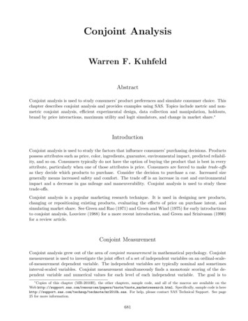
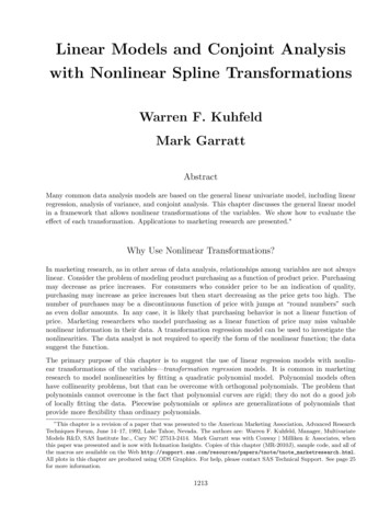
1216MR-2010J — Linear Models and Conjoint Analysis with Nonlinear Spline TransformationsFigure 1. Linear, Quadratic, and Cubic CurvesFigure 2. Curves For Knots at 2, 0, 2from the linear modely β0 β1 x β2 x2 β3 x3 is a cubic spline with no knots. This equation models y as a nonlinear function of x, but does sowith a linear regression model; y is a linear function of x, x2 , and x3 . Table 1 shows the X matrix,(1 x x2 x3 ), for a cubic polynomial, where x 5, 4, ., 5. Figure 1 plots the polynomial terms(except the intercept). See Smith (1979) for an excellent introduction to splines.Splines with KnotsHere is an example of a polynomial spline model with three knots at t1 , t2 , and t3 .y β0 β1 x β2 x2 β3 x3 β4 (x t1 )(x t1 )3 β5 (x t2 )(x t2 )3 β6 (x t3 )(x t3 )3 The Boolean expression (x t1 ) is 1 if x t1 , and 0 otherwise. The termβ4 (x t1 )(x t1 )3is zero when x t1 and becomes nonzero, letting the curve change, as x becomes greater than knot t1 .This spline uses more df and is less smooth than the polynomial modely β0 β1 x β2 x2 β3 x3 Assume knots at 2, 0, and 2; the spline model is:y β0 β1 x β2 x2 β3 x3
MR-2010J — Linear Models and Conjoint Analysis with Nonlinear Spline TransformationsFigure 3. A Spline Curve With Knots at 2, 0, 21217Figure 4. The Components of the Splineβ4 (x 2)(x 2)3 β5 (x 0)(x 0)3 β6 (x 2)(x 2)3 Table 2 shows an X matrix for this model, Figure 1 plots the polynomial terms, and Figure 2 plots theknot terms.The β0 , β1 x, β2 x2 , and β3 x3 terms contribute to the overall shape of the curve. Theβ4 (x 2)(x 2)3term has no effect on the curve before x 2, and allows the curve to change at x 2. Theβ4 (x 2)(x 2)3 term is exactly zero at x 2 and increases as x becomes greater than 2. Theβ4 (x 2)(x 2)3 term contributes to the shape of the curve even beyond the next knot at x 0,but at x 0,β5 (x 0)(x 0)3allows the curve to change again. Finally, the last termβ6 (x 2)(x 2)3allows one more change. For example, consider the curve in Figure 3. It is the spliney 0.5 0.01x 0.04x2 0.01x3 0.1(x 2)(x 2)3 0.5(x 0)(x 0)3 1.5(x 2)(x 2)3It is constructed from the curves in Figure 4. At x 2.0 there is a branch;y 0.5 0.01x 0.04x2 0.01x3
1218MR-2010J — Linear Models and Conjoint Analysis with Nonlinear Spline Transformationscontinues over and down while the curve of interest,y 0.5 0.01x 0.04x2 0.01x3 0.1(x 2)(x 2)3starts heading upwards. At x 0, the addition of 0.5(x 0)(x 0)3slows the ascent until the curve starts decreasing again. Finally, the addition of1.5(x 2)(x 2)3produces the final change. Notice that the curves do not immediately diverge at the knots. Thefunction and its first two derivatives are continuous, so the function is smooth everywhere.Derivatives of a Polynomial SplineThe next equations show a cubic spline model with a knot at t1 and its first three derivatives withrespect to x.y β0 β1 x β2 x2 β3 x3 β4 (x t1 )(x t1 )3 dydx β1 2β2 x 3β3 x2 3β4 (x t1 )(x t1 )2d2 ydx2 2β2 6β3 x 6β4 (x t1 )(x t1 )d3 ydx3 6β3 6β4 (x t1 )The first two derivatives are continuous functions of x at the knots. This is what gives the splinefunction its smoothness at the knots. In the vicinity of the knots, the curve is continuous, the slope ofthe curve is a continuous function, and the rate of change of the slope function is a continuous function.The third derivative is discontinuous at the knots. It is the horizontal line 6β3 when x t1 and jumpsto the horizontal line 6β3 6β4 when x t1 . In other words, the cubic part of the curve changes atthe knots, but the linear and quadratic parts do not change.
MR-2010J — Linear Models and Conjoint Analysis with Nonlinear Spline TransformationsFigure 5. A Discontinuous Spline Function1219Figure 6. A Spline With a Discontinuous SlopeDiscontinuous Spline FunctionsHere is an example of a spline model that is discontinuous at x t1 .y β0 β1 x β2 x2 β3 x3 β4 (x t1 ) β5 (x t1 )(x t1 ) β6 (x t1 )(x t1 )2 β7 (x t1 )(x t1 )3 Figure 5 shows an example, and Table 3 shows a design matrix for this model with t1 0. The fifthcolumn is a binary (zero/one) vector that allows the discontinuity. It is a change in the interceptparameter. Note that the sixth through eighth columns are necessary if the spine is to consist of twoindependent polynomials. Without them, there is a jump at t1 0, but both curves are based on thesame polynomial. For x t1 , the spline isy β0 β1 x β2 x2 β3 x3 and for x t1 , the spline isy β0 β4 β1 x β5 (x t1 ) β2 x2 β6 (x t1 )2 β3 x3 β7 (x t1 )3 The discontinuities are as follows:β7 (x t1 )(x t1 )3specifies a discontinuity in the third derivative of the spline function at t1 ,β6 (x t1 )(x t1 )2
1220MR-2010J — Linear Models and Conjoint Analysis with Nonlinear Spline TransformationsTable 4Cubic B-Spline With Knots at 2, 0, 40.301.00Figure 7. B-Splines With Knots at 2, 0, 2specifies a discontinuity in the second derivative at t1 ,β5 (x t1 )(x t1 )specifies a discontinuity in the derivative at t1 , andβ4 (x t1 )specifies a discontinuity in the function at t1 . The function consists of two separate polynomial curves,one for x t1 and the other for t1 x . This kind of spline can be used to model adiscontinuity in price.Here is an example of a spline model that is continuous at x t1 but does not have d 1 continuousderivatives.y β0 β1 x β2 x2 β3 x3 β4 (x t1 )(x t1 ) β5 (x t1 )(x t1 )2 β6 (x t1 )(x t1 )3 dydx β1 2β2 x 3β3 x2 β4 (x t1 ) 2β5 (x t1 )(x t1 ) 3β6 (x t1 )(x t1 )2Since the first derivative is not continuous at t1 x, the slope of the spline is not continuous at t1 x.Figure 6 contains an example with t1 0. Notice that the slope of the curve is indeterminate at zero.
MR-2010J — Linear Models and Conjoint Analysis with Nonlinear Spline Transformations1221Table 5Polynomial and B-Spline EigenvaluesPolynomial Spline BasisB-Spline 99971.000001.00000Monotone Splines and B-SplinesAn increasing monotone spline never decreases; its slope is always positive or zero. Decreasing monotonesplines, with slopes that are always negative or zero, are also possible. Monotone splines cannot beconveniently created from polynomial splines. A different basis, the B-spline basis, is used instead.Polynomial splines provide a convenient way to describe splines, but B-splines provide a better way tofit spline models.The columns of the B-spline basis are easily constructed with a recursive algorithm (de Boor 1978,pages 134–135). A basis for a vector space is a linearly independent set of vectors; every vector in thespace has a unique representation as a linear combination of a given basis. Table 4 shows the B-splineX matrix for a model with knots at 2, 0, and 2. Figure 7 shows the B-spline curves. The columnsof the matrix in Table 4 can all be constructed by taking linear combinations of the columns of thepolynomial spline in Table 2. Both matrices form a basis for the same vector space.The numbers in the B-spline basis are all between zero and one, and the marginal sums across columnsare all ones. The matrix has a diagonally banded structure, such that the band moves one position tothe right at each knot. The matrix has many more zeros than the matrix of polynomials and muchsmaller numbers. The columns of the matrix are not orthogonal like a matrix of orthogonal polynomials,but collinearity is not a problem with the B-spline basis like it is with a polynomial spline. The B-splinebasis is very stable numerically.To illustrate, 1000 evenly spaced observations were generated over the range -5 to 5. Then a B-splinebasis and polynomial spline basis were constructed with knots at 2, 0, and 2. The eigenvalues forthe centered X0 X matrices, excluding the last structural zero eigenvalue, are given in Table 5. In thepolynomial splines, the first two components already account for more than 99% of the variation ofthe points. In the B-splines, the cumulative proportion does not pass 99% until the last term. Theeigenvalues show that the B-spline basis is better conditioned than the piecewise polynomial basis.B-splines are used instead of orthogonal polynomials or Box-Cox transformations because B-splinesallow knots and more general curves. B-splines also allow monotonicity constraints.
1222MR-2010J — Linear Models and Conjoint Analysis with Nonlinear Spline TransformationsA transformation of x is monotonically increasing if the coefficients that are used to combine thecolumns of the B-spline basis are monotonically increasing. Models with splines can be fit directlyusing ordinary least squares (OLS). OLS does not work for monotone splines because OLS has nomethod of ensuring monotonicity in the coefficients. When there are monotonicity constraints, analternating least square (ALS) algorithm is used. Both OLS and ALS attempt to minimize a squarederror loss function. See Kuhfeld (1990) for a description of the iterative algorithm that fits monotonesplines. See Ramsay (1988) for some applications and a different approach to ensuring monotonicity.Transformation RegressionIf the dependent variable is not transformed and if there are no monotonicity constraints on theindependent variable transformations, the transformation regression model is the same as the OLSregression model. When only the independent variables are transformed, the transformation regressionmodel is nothing more than a different rendition of an OLS regression. All of the spline models presentedup to this point can be reformulated asy β0 Φ(x) The nonlinear transformation of x is Φ(x); it is solved for by fitting a spline model such asy β0 β1 x β2 x2 β3 x3 β4 (x t1 )(x t1 )3 β5 (x t2 )(x t2 )3 β6 (x t3 )(x t3 )3 whereΦ(x) β1 x β2 x2 β3 x3 β4 (x t1 )(x t1 )3 β5 (x t2 )(x t2 )3 β6 (x t3 )(x t3 )3Consider a model with two polynomials:y β0 β1 x1 β2 x21 β3 x31 β4 x2 β5 x22 β6 x32 It is the same as a transformation regression modely β0 Φ1 (x1 ) Φ2 (x2 ) where Φ ( ) designates cubic spline transformations with no knots. The actual transformations in thiscase areb 1 (x1 ) βb1 x1 βb2 x2 βb3 x3Φ11andb 2 (x2 ) βb4 x2 βb5 x2 βb6 x3Φ22There are six model df. The test for the effect of the transformation Φ1 (x1 ) is the test of the linearhypothesis β1 β2 β3 0, and the Φ2 (x2 ) transformation test is a test that β4 β5 β6 0.Both tests are F-tests with three numerator df. When there are monotone transformations, constrainedleast-squares estimates of the parameters are obtained.
MR-2010J — Linear Models and Conjoint Analysis with Nonlinear Spline Transformations1223Degrees of FreedomIn an ordinary general linear model, there is one parameter for each independent variable. In thetransformation regression model, many of the variables are used internally in the bases for the transformations. Each linearly independent basis column has one parameter and one model df. If a variableis not transformed, it has one parameter. Nominal classification variables with c categories have c 1parameters. For degree d splines with k knots and d 1 continuous derivatives, there are d kparameters.When there are monotonicity constraints, counting the number of scoring parameters is less precise.One way of handling a monotone spline transformation is to treat it as if it were simply a splinetransformation with d k parameters. However, there are typically fewer than d k unique parameterestimates since some of those d k scoring parameter estimates may be tied to impose the orderconstraints. Imposing ties is equivalent to fitting a model with fewer parameters. So, there are twoavailable scoring parameter counts: d k and a potentially smaller number that is determined duringthe analysis. Using d k as the model df is conservative since the scoring parameter estimates arerestricted. Using the smaller count is too liberal since the data and the model together are being used todetermine the number of parameters. Our solution is to report tests using both liberal and conservativedf to provide lower and upper bounds on the “true” p-values.Dependent Variable TransformationsWhen a dependent variable is transformed, the problem becomes multivariate:Φ0 (y) β0 Φ1 (x1 ) Φ2 (x2 ) Hypothesis tests are performed in the context of a multivariate linear model, with the number of dependent variables equal to the number of scoring parameters for the dependent variable transformation.Multivariate normality is assumed even though it is known that the assumption is always violated.This is one reason that all hypothesis tests in the presence of a dependent variable transformationshould be considered approximate at best.For the transformation regression model, we redefine three of the usual multivariate test statistics:Pillai’s Trace, Wilks’ Lambda, and the Hotelling-Lawley Trace. These statistics are normally computedusing all of the squared canonical correlations, which are the eigenvalues of the matrix H(H E) 1 .Here, there is only one linear combination (the transformation) and hence only one squared canonicalcorrelation of interest, which is equal to the R2 . We use R2 for the first eigenvalue; all other eigenvaluesare set to zero since only one linear combination is used. Degrees of freedom are computed assumingthat all linear combinations contribute to the Lambda and Trace statistics, so the F-tests for thosestatistics are conservative. In practice, the adjusted Pillai’s Trace is very conservative—perhaps tooconservative to be useful. Wilks’ Lambda is less conservative, and the Hotelling-Lawley Trace seemsto be the least conservative.It may seem that the Roy’s Greatest Root statistic, which always uses only the largest squared canonicalcorrelation, is the only statistic of interest. Unfortunately, Roy’s Greatest Root is very liberal and onlyprovides a lower bound on the p-value. The p-values for the liberal and conservative statistics are usedtogether to provide approximate lower and upper bounds on p.
1224MR-2010J — Linear Models and Conjoint Analysis with Nonlinear Spline TransformationsScales of MeasurementEarly work in scaling, such as Young, de Leeuw, & Takane (1976), and Perreault & Young (1980)was concerned with fitting models with mixed nominal, ordinal, and interval scale of measurementvariables. Nominal variables were optimally scored using Fisher’s (1938) optimal scoring algorithm.Ordinal variables were optimally scored using the Kruskal and Shepard (1974) monotone regressionalgorithm. Interval and ratio scale of measurement variables were left alone nonlinearly transformedwith a polynomial transformation.In the transformation regression setting, the Fisher optimal scoring approach is equivalent to using anindicator variable representation, as long as the correct df are used. The optimal scores are categorymeans. Introducing optimal scaling for nominal variables does not lead to any increased capability inthe regression model.For ordinal variables, we believe the Kruskal and Shepard monotone regression algorithm should bereserved for the situation when a variable has only a few categories, say five or fewer. When there aremore levels, a monotone spline is preferred because it uses fewer model df and because it is less likelyto capitalize on chance.Interval and ratio scale of measurement variables can be left alone or nonlinearly transformed withsplines or monotone splines. When the true model has a nonlinear function, sayy β0 β1 log(x) ory β0 β1 /x the transformation regression modely β0 Φ(x) bcan be used to hunt for parametric transformations. Plots of Φ(x)may suggest log or reciprocaltransformations.Conjoint AnalysisGreen & Srinivasan (1990) discuss some of the problems that can be handled with a transformationregression model, particularly the problem of degrees of freedom. Consider a conjoint analysis designwhere a factor with c 3 levels has an inherent ordering. By finding a quadratic monotone splinetransformation with no knots, that variable will use only two df instead of the larger c 1. Themodel df in a spline transformation model are determined by the data analyst, not by the numberof categories in the variables. Furthermore, a “quasi-metric” conjoint analysis can be performed byfinding a monotone spline transformation of the dependent variable. This model has fewer restrictionsthan a metric analysis, but will still typically have error df, unlike the nonmetric analysis.
MR-2010J — Linear Models and Conjoint Analysis with Nonlinear Spline Transformations1225Curve Fitting ApplicationsWith a simple regression model, you can fit a line through a y x scatter plot. With a transformationregression model, you can fit a curve through the scatter plot. The y-axis coordinates of the curve arebyb βb0 Φ(x)from the modely β0 Φ(x) With more than one group of observations and a multiple regression model, you can fit multiple lines,lines with the same slope but different intercepts, and lines with common intercepts but different slopes.With the transformation regression model, you can fit multiple curves through a scatter plot. Thecurves can be monotone or not, constrained to be parallel, or constrained to have the same intercept.Consider the problem of modeling the number of product purchases as a function of price. Separatecurves can be simultaneously fit for two groups who may behave differently, for example those who aremaking a planned purchase and those who are buying impulsively. Later in this chapter, there is anexample of plotting brand by price interactions.Figure 8 contains an artificial example of two separate spline functions; the shapes of the two curvesare independent of each other, and R2 0.87. In Figure 9, the splines are constrained to be parallel,and R2 0.72. The parallel curve model is more restrictive and fits the data less well than theunconstrained model. In Figure 8, each curve follows its swarm of data. In Figure 9, the curves findpaths through the data that are best on the average considering both swarms together. In the vicinityof x 2, the top curve is high and the bottom curve is low. In the vicinity of x 1, the top curveis low and the bottom curve is high.Figure 10 contains the same data and two monotonic spline functions; the shapes of the two curves areindependent of each other, and R2 0.71. The top curve is monotonically decreasing, whereas the bottom curve is monotonically increasing. The curves in Figure 10 flatten where there is nonmonotonicityin Figure 8.Parallel curves are very easy to model. If there are two groups and the variable g is a binary variableindicating group membership, fit the modely β0 β1 g Φ1 (x) where Φ1 (x) is a linear, spline, or monotone spline transformation. Plot yb as a function of x to see thetwo curves. Separate curves are almost as easy; the model isy β0 β1 g Φ1 (x (1 g)) Φ2 (x g) When x (1 g) is zero, x g is x, and vice versa.
1226MR-2010J — Linear Models and Conjoint Analysis with Nonlinear Spline TransformationsFigure 8. Separate Spline Functions, Two GroupsFigure 10. Monotone Spline Functions, Two GroupsFigure 9. Parallel Spline Functions, Two Groups
MR-2010J — Linear Models and Conjoint Analysis with Nonlinear Spline Transformations1227Spline Functions of PriceThis section illustrates splines with an artificial data set. Imagine that subjects were asked to rate theirinterest in purchasing various types of spaghetti sauces on a one to nine scale, where nine indicateddefinitely will buy and one indicated definitely will not buy. Prices were chosen from typical retailtrade prices, such as 1.49, 1.99, 2.49, and 2.99; and one penny more than a typical price, 1.00, 1.50, 2.00, and 2.50. Between each “round” number price, such as 1.00, and each typical price,such as 1.49, three additional prices were chosen, such as 1.15, 1.25, and 1.35. The goal is to allowa model with a separate spline for each of the four ranges: 1.00 — 1.49, 1.50 — 1.99, 2.00 — 2.49, and 2.50 — 2.99. For each range, a spline with zero or one knot can be fit.One rating for each price was constructed and various models were fit to the data. Figures 11 through18 contain results. For each figure, the number of model df are displayed. One additional df for theintercept is also used. The SAS/STAT procedure TRANSREG was used to fit all of the models in thischapter.Figure 11 shows the linear fit, Figure 12 uses a quadratic polynomial, and Figure 13 uses a cubicpolynomial. The curve in Figure 13 has a slight nonmonotonicity in the tail, and since it is a polynomial,it is rigid and cannot locally fit the data values.Figure 14 shows a monotone spline. It closely follows the data and never increases. A range for themodel df is specified; the larger value is a conservative count and the smaller value is a liberal count.The curves in Figures 12 through 14 are all continuous and smooth. These curves do a good job offollowing the data, but inspection of the data suggests that a different model may be more appropriate.There is a large drop in purchase interest when price increases from 1.49 to 1.50, a smaller dropbetween 1.99 and 2.00, and a still smaller drop between 2.49 and 2.50.In Figure 15, a separate quadratic polynomial is fit for each of the four price ranges: 1.00 — 1.49, 1.50 — 1.99, 2.00 — 2.49, and 2.50 — 2.99. The functions are
analysis of variance model, or a metric conjoint analysis model. The model y β 0 β 1x β 2x2 β 3x3 is of special interest. It is a linear model because it is linear in the parameters, and it models y as a nonlinear function of x. It is a cubic polynomial regression model, which is a special case of a spline. Polynomial Splines