Transcription
Optical Lithography Modelling with MATLAB Laboratory Manualto accompanyFundamentalPrinciples of OpticalLithography, byChris Mack20112011Optical LithographyModelling with MATLAB Kevin Berwick
Optical Lithography Modelling with MATLAB 2011ContentsForeword . 2Preface . 31. Introduction to Semiconductor Lithography . 52. Aerial Image Formation – The Basics . 93. Aerial Image Formation – The Details . 134. Imaging in Resist: Standing Waves and Swing Curves . 235. Conventional Resists: Exposure and Bake Chemistry . 306. Chemically Amplified Resists: Exposure and Bake Chemistry . 387. Photoresist Development . 438. Lithographic Control in Semiconductor Manufacturing . 499. Gradient-Based Lithographic Optimization: Using the Normalized Image Log-Slope 5310. Resolution Enhancement Technologies . 57A MATLAB Primer . 60This work is licenced under a Creative Commons Licence.Kevin BerwickPage 1
Optical Lithography Modelling with MATLAB 2011ForewordLike virtually any area of study, optical lithography is best learned by acombination of thinking and doing. Reading my textbook, FundamentalPrinciples of Optical Lithography, will certainly require a fair amount ofthinking. And doing the homework problems is a first step in “doing”, practicinglithography to reinforce the concepts found in the book. But the real practice oflithography – getting in the fab or lab and printing wafers – is often out of thereach of most students, requiring equipment and facilities that are frequentlyunavailable. Thus, there is a need for more opportunities to “do” than the book’shomework problems can provide. Simulating lithography, performing thecomplex calculations detailed in my book to create a virtual lithographyenvironment, is a valuable way to get experiences closer to the real world oflithography practice without the (sometimes extreme) expense of physicalexperiments.While sophisticated lithography simulators such as PROLITH are extremelyvaluable learning tools for the student of lithography, Kevin Berwick in thisvolume offers another approach to learning through simulation: use the power ofthe MATLAB environment to enable students to write their own code forperforming complex lithography calculations. Found within these pages arelaboratory “experiments” to be performed in the MATLAB environment. Theyare, in a sense, extreme homework problems, requiring computationalcapabilities that often stretch far beyond paper, pencil and calculator. But theirvery complexity enables a new level of learning – the ability to toy with inputsand examine the resulting outputs in a simulated lithography experience. Whileseeing a graph showing how an output varies with an input can be instructive,doing the calculations that generate that curve is even more instructive. KevinBerwick’s MATLAB laboratory manual is a valuable resource for the reader ofFundamental Principles of Optical Lithography. Whether in academia or inindustry, performing the laboratories found in this manual will bring one’slithography learning a little closer to reality.Chris MackDecember, 2010Austin, Texas, USAKevin BerwickPage 2
Optical Lithography Modelling with MATLAB 2011PrefaceThe original motivation to write this book was when I was asked to teach anelective, one-semester course in Lithography as part of a new M. Sc. Program atthe Dublin Institute of Technology. While there are many books available whichdescribe the full range of processes required to build a circuit on silicon, very fewexist which concentrate solely on Lithography.One of the aspects of Lithography which I wanted to highlight was mathematicalmodelling of Lithography and, as I searched the literature in order to findinformation on this for my lecture notes, Chris Mack’s name cropped up againand again. As the author of the lithography simulation software PROLITH ,Chris has an enormous breadth of knowledge on the subject of lithographymodelling. I was delighted when, in 2007, Chris’s book, Fundamental Principlesof Optical Lithography, was published. Here was a synthesis of the many, manypapers published in the field, filtered by an expert and dished up in an easilydigestible form for my reading pleasure.For about a month, my morning routine before starting my teaching consisted ofa train journey into town, followed by two double shot lattes at Insomnia, myfavourite coffee shop, as I read Chris’s book from cover to cover. Themathematics was, in parts, intimidating. Although largely standard algebra andcalculus, many of the expressions developed were long. In addition, theinterpretation of the mathematics was challenging, requiring me to dust off someof the physics I hadn’t used for the best part of a decade. As an engineer, I foundthat the plots of the equations in the text were a great help in visualising theunderlying physics.Initially, I wrongly assumed that all the plots had been generated usingPROLITH . However, as I read further, it became apparent that most of theFigures could be reproduced with any mathematical calculation and plottingprogram.Coincidentally, I had started to use MATLAB for teaching several other subjectsaround this time. MATLAB allows you to develop mathematical modelsquickly, using powerful language constructs, and is used in almost everyEngineering School on Earth. MATLAB has a particular strength in datavisualisation, allowing you to get insight into trends in data far quicker than usingspreadsheets or other high level languages such as C or Fortran. I decided toattempt to reproduce some of the plots in Chris’s book using MATLAB and stillremember my delight when, after writing only a few lines of MATLAB code, anAerial Image plot identical to that in the book materialised on my screen.In my experience, familiarity with theoretical models, and the underlyingphysical principles used in constructing the models, is greatly improved if thebehaviour of the equations is explored using computer software. So, I wroteseveral laboratory exercises for my students based on Chris’s book usingMATLAB . The lab sheets I produced eventually grew into the book you are nowreading.Kevin BerwickPage 3
Optical Lithography Modelling with MATLAB 2011This book is intended to act as a companion to Chris’s book, reinforcing theprinciples covered in the text. As such, I would imagine the Manual will proveuseful to Senior Undergraduate and Graduate students, as well as practisinglithographers who wish to improve their theoretical knowledge of what isessentially a practical process. Along the way, the interested student will gainsome familiarity with MATLAB . In order to kick start this process, I include ashort MATLAB Primer as an Appendix to the text.An Instructor’s Solution manual is available by emailing me atkevin.berwick@dit.ie . Suggestions for improvements, error reports and additionsto the book are always welcome and can be sent to me at this email address.I would like to thank a number of people who assisted in the production of thismanual. I have already mentioned Chris Mack, author of Fundamental Principlesof Optical Lithography. Most of the questions in this Manual are based directlyon his textbook. Chris advised me on the mathematics and physics when needed,and supplied me with analytical solutions to many of the problems. He alsoprovided valuable advice at various stages of the production of the book and hisenthusiasm for the project when initially proposed was very encouraging.I also received valuable feedback from anonymous reviewers during the writingof the book and am very grateful for their contributions. I would like to thank TheMathWorks for their support via their Book program and for producing theMATLAB software on which this book is based. I would also like to thank theSchool of Electronics and Communications Engineering at the Dublin Institute ofTechnology for affording me the opportunity to write this book.Finally, I would like to thank my family, who tolerated my absence on the manyoccasions when, largely self imposed, deadlines loomed.Kevin BerwickDublin, IrelandDecember 2010Kevin BerwickPage 4
Optical Lithography Modelling with MATLAB 20111. Introduction to Semiconductor Lithography1. Plot the projected range and straggle for the ion implantation of Boron into resist. Usethe data in Table 1.1 of the Book. You should get something like this.3000Projected Range 800Ion Energy (keV)1000120014001600600800Ion Energy (keV)1000120014001600200Straggle (nm)150100SSPPEECCIIMMEENN5000200400(i) What energy is required to produce a Boron implant with a projected range of 1μm?(ii) What is the straggle at this Energy?2. The Yield, Production Cost and Profit, in dollars, of a chip at a semiconductor plantcan be described by(1.3)where w is the feature size in nm, (which must be greater than w0, the ultimate resolution,in this model), and σ is the sensitivity of Yield to feature size. If w0 65 nm and σ 9nm, plot Yield, Production Cost and Profit as a function of feature size, for feature sizesbetween 72 nm and 120 nm.Kevin BerwickPage 5
Optical Lithography Modelling with MATLAB 2011You should get something like this.109Chip Yield0.80.7Chip Production Cost ( 859095100105Minimum feature size 0105Minimum feature size (nm)1101151205Profit per chip ( m feature size (nm)Answer the following questions.(i) Below what feature size does the Yield drop below 30%?(ii) Above what feature size does the Yield exceed 95%?(iii) What is the feature size at the lowest Production Cost?(iv) What is the Yield at the lowest Production Cost?(v) What is the maximum Profit per chip, in dollars, at this plant?(vi) What is the feature size when the plant is most profitable?(vii) What is the Yield when the plant is most profitable?3. Resolution in optical lithography scales with wavelength, λ, and numerical aperture,NA, according to a modified Rayleigh criterion:where k1 can be thought of as a constant for a given lithographic approach and process.Assuming k1 0.35, plot resolution versus numerical aperture over a range of NAs from0.5 to 1.0 for the common lithographic wavelengths of 436 nm, 365 nm, 248 nm, 193 nm,and 157 nm. From this list, what options (NA and wavelength) are available for printing90 nm features? Your plot should look like this.Kevin BerwickPage 6
Optical Lithography Modelling with MATLAB 2011Resolution vs IIMMEENN1005000.50.60.70.80.9NA11.11.21.34. Resist thickness scales as(1.4)ω is the spin speed and υ is the resist viscosity. If k is the constant of proportionality.The Reynold’s number, Re, is given by(1.5)where r is the wafer radius and υair is the viscosity of air.(i) Plot thickness of resist as a function of resist viscosity for viscosities of 5 – 35 cStoke(1 Stoke 1 cm2/s), for a spin speed of 2000 rpm. Take care with dimensions, assumingk 4.38 x 10⁻⁴, υ is in m2/s and ω is in revolutions per second.(ii) Plot the Reynolds number as a function of spin speed for a 300 mm wafer and provethat a spin speed of 2000 rpm will not cause turbulent flow, given that flow instabilitieswould be expected to begin at a Reynolds number of 100,000. Take υair 1.56 x 10⁻⁵m2/s.(iii) Plot thickness of resist as a function of spin speed, for a resist viscosity of 20cStokes, for spin speeds between 2000 and 5000 rpm.Kevin BerwickPage 7
Optical Lithography Modelling with MATLAB 2011You should get something like the plots shown.41.314x 10121.1Reynolds numberResist thickness MMEENN860.60.5510152025Resist viscosity (c Stokes)303545005000420002500300035004000Spin speed (rpm)45005000Resist thickness (microns)1.110.90.8SSPPEECCIIMMEENN0.72000Kevin Berwick2500300035004000Spin speed (rpm)Page 8
Optical Lithography Modelling with MATLAB 20112. Aerial Image Formation – The BasicsAerial Image calculation: - Dense Lines and Spaces1. This exercise is based on Chapter 2 of the book, in particular the material presented inSection 2.2.5. In this exercise, we will look at the aerial image formed by a dense patternof lines and spaces as a function of the number of diffraction orders captured by theobjective lens. We will assume coherent illumination is used.The diffraction pattern of an infinite array of lines and spaces is made up of discretediffraction orders, mathematically represented by delta functions. The image of such apattern is calculated as the Inverse Fourier Transform of the diffraction orders that makeit through the lens, that is, those with spatial frequencies less than NA/λ.We can show that for a dense array of lines and spacesE(x) a0 (2πjx/p)(2.63)The zeroth order, given by a0, provides a DC offset to the electric field. Each pair ofdiffraction orders j /- 1, 2, 3, etc., contributes a cosine at harmonics of the pitch p tothe image. In order to calculate the coefficients ,aj (2.62)where w is the linewidth and p is the pitch. The Electric Field Intensity is given byI (x) n(2.39)Take n 1 for this exercise, that is, assume that the medium is air.2. For equal lines and spaces, calculate a1 to a11. How can a0 be calculated?3. Write a MATLAB program to calculate the Aerial image, that is, the Electric FieldIntensity, I(x), across a space, as a function of the number of diffraction orders capturedby the objective lens. Assume coherent illumination is used for a pattern of equal linesand spaces of width 500 nm and an associated pitch of 1000 nm. Do the calculation for N 1, 3, 5, 7, 9, 11.Kevin BerwickPage 9
Optical Lithography Modelling with MATLAB 20111.4N 1N 3N 5N 7N 9N 111.2SSPPEECCIIMMEENNRelative ntal position nm100200300400500You should get a plot which looks like the one above.4. If you repeated the exercise, but this time included even diffracted orders, that is, N 2, 4, 6, 8 etc., how would the results be affected?5. Do a hand calculation of the intensity at the centre of the space (x 0) and the centreof a line (x p/2) for the case where N 1, that is, 3-beam imaging. Does it match theresults from your MATLAB simulation?6. Note that as the number of orders captured by the lens, that is, the NA, increases, theimage improves. The ringing in the image is reduced, while the transition from dark tolight is sharper. Ideally, you want to collect as many diffracted orders as possible, that is,have a large NA. If a wavelength of 248 nm is used to image this dense pattern of linesand spaces, and given that on-axis, coherent illumination is used, calculate whichdiffraction orders pass through the lens. Take the numerical aperture of the lens to be0.85. Plot the image using MATLAB .7. In the text, Section 2.3.1, it says that oblique illumination results in a shift of thediffraction pattern by an amount, in spatial frequency terms, of sin θ'/λ. If the illuminationsystem in the stepper described earlier is tilted by an angle of 30 degrees, identify whichdiffraction orders get through to the lens.Kevin BerwickPage 10
Optical Lithography Modelling with MATLAB 2011Partially coherent illumination, the Kintner method1. This Exercise is based on Chapter 2 of the book, in particular the material presented inSection 2.3.2.Mask Pattern(equal lines and spaces)Diffraction PatternLens ApertureFigure 2.15 The diffraction pattern is broadened by the use of partially coherent illumination(plane waves over a range of angles striking the mask)If the mask illumination comes from a range of angles, rather than just one, we say thelight is partially coherent.For a uniform intensity, circular source and a repeating pattern of lines and spaces, theaerial image is given byI ( x) s I 1 beam s 2 I 2 beam s I 3 beam13(2.90)where s1, s2, and s3 are given in Table 2.3 and(2.91)(2.92)(2.93)Kevin BerwickPage 11
Optical Lithography Modelling with MATLAB 2011Table 2.3 Kintner weights for conventional source imaging of small lines and spaces.Regime pNADescriptions2s3All 3-beam imaging001Combination of two- andthree-beam imaging02 1 – 2 Combination of one-, twoand three-beam imaging 2 – 12(1 – – ) 2 – 12(1 – )0100 1 1 pNA1 2 1 s1 pNA1 1 2 pNA 1Combination of one- andtwo-beam imaging 1 Only the zero order iscaptured, all 1-beampNAIn this Exercise, we will calculate the aerial image formed by a dense pattern of lines andspaces formed using partially coherent illumination.2. Read pp 58-62 in Fundamental Principles of Optical Lithography, by Chris Mack.3. Write a MATLAB program to calculate the Aerial image, that is, the Electric FieldIntensity, I(x), across a space. Assume partially coherent, 248 nm illumination withvalues of σ 0.8, NA 0.8 and the linewidth spacewidth 200 nm. Note that thisinvolves plotting Eq (2.90). You should get a plot which looks like the one below.2SSppeecciimmeennRelative Intensity1.510.50-0.5-200-150Kevin Berwick-100-500Horizontal position (nm)50100150200Page 12
Optical Lithography Modelling with MATLAB 20113. Aerial Image Formation – The Details1. Plot the Z3, Z4, Z6 and Z8 Zernike formulae using MATLAB . You should getsomething like 0.50-0.5-110.50-0.5-1-0.5-110.50-0.5-12. Equation (3.6) describes 3rd order x coma asZ6(3.6)For simplicity, we consider coma in the direction of maximum magnitude is given by Eq(3.6) with cmaximum, that is 1. From Table 3.1, Z1is the x-tilt. Comparingthese Equations, we see that coma acts as an x- tilt with coefficient. Thisleads to a placement error which varies with R.We know that tilt generates a placement error ofPlacement error (3.5)By comparison, we would expect coma to generate a placement error ofPlacement error Kevin BerwickPage 13
Optical Lithography Modelling with MATLAB 2011Consider a pattern of lines and spaces of pitch p. Diffraction will produce discrete ordersof light passing through the lens. The zeroth order goes straight through the lens centre,while the first orders enter the lens at radial positions. The placement erroris given by substituting R into the Equation for placement error as a result ofComa above.Placement error (3.7)This applies to line/space patterns and λ/NA p 3λ/NA and coherent illumination. Itpredicts that you will get a negative placement error when the pitch is less than 1.5λ/NA,a positive error for pitches greater than this amount, and zero placement error when thepitch is equal to this amount.The error is zero when, other values of R will sufferplacement error. Show why this is true, using plots of the wavefront error generatedusing MATLAB .You should get something like this for your plot of wavefront error.10.8X: 0.95Y: 0.67210.6negative tiltX: -0.65Y: 0.4761positive tiltWavefront error (arb -units)0.40.2SSPPEECCIIMMEENNno tilt0-0.2X: 0.65Y: -0.4761-0.4-0.6X: -0.95Y: -0.6721-0.8-1-1Kevin Berwick-0.8-0.6-0.4-0.20Relative pupil position0.20.40.60.81Page 14
Optical Lithography Modelling with MATLAB 20113. Consider the case of dense equal lines and spaces (only the 0 and 1st orders are used)imaged with coherent TE illumination. Using MATLAB , plot the aerial image intensityfor this situation, given by Eq (3.27). By changing the amount of defocus over a suitablerange, show that the peak intensity of the image in the middle of the space falls offapproximately quadratically with defocus, for small amounts of defocus. Here is sometypical data, together with a fit generated using MATLAB .DefocusIntensity01.290.05π1.2840.1 π1.260.15 π1.220.2 π1.17SSPPEECCIIMMEENNKevin BerwickPage 15
Optical Lithography Modelling with MATLAB 20114. Compare the depth of focus predictions of the high-NA version of the Rayleighequation (3.60) to the paraxial version of equation (3.61) by plotting predicted DOFversus pitch. Use k2 0.6, λ 248 nm and pitches in the range from 250 to 500 nm.Assume imaging in air.DOF (high NA)(3.60)DOF (low NA) k2(3.61)You should get something like this plot.700Low NAHigh NA600Rayleigh DOF 00Pitch nm5. Read Section 3.6.2. Note that for TE illumination, and for a y - oriented dense pattern,the electric field component for TE polarisation is in the y - direction. However, TMillumination has x- and z- components present, and will give a degraded image whencompared to that produced by TE illumination.Consider the case of dense equal lines and spaces (only the 0 and 1st orders are used),with the linewidth and spacewidth equal to 250 nm, imaged with conventional coherentillumination at a wavelength of λ 193 nm. Explore the influence of polarisation of theillumination source by plotting both the TE and TM aerial images.You should get something like this.Kevin BerwickPage 16
Optical Lithography Modelling with MATLAB .20-250-200-150-100-500horizontal position501001502002506. In this exercise, we will look at the effect of defocus on a pattern of lines and spacesformed by a projection lithography system utilizing the 0 and /-1 diffraction orders only,that is, 3-beam imaging using coherent illumination and TE polarization.The intensity image in this case is given byI(x) (3.27)The impact of defocus is to reduce the magnitude of the main cosine term in the image.As the first orders go out of phase with respect to the zeroth order, the interferencebetween the zeroth and first orders decreases. When 900, there is no interferenceand theterm disappears. For defocus δ we get(3.25)Note that for coherent imaging, 0.Consider a coherent, three-beam image of a line/space pattern under TE illumination.NA 0.93, λ 193 nm, linewidth 100 nm, spacewidth 150, pitch 250 nm. Plot theresulting aerial image at best focus and at defocus values of 50 and 100 nm for:i) imaging in airii) immersion imaging in a fluid with a refractive index of 1.44.Kevin BerwickPage 17
Optical Lithography Modelling with MATLAB 2011You should get something like this for imaging in air.1.5defocus 0defocus 50defocus 1001Intensity a.uSSPPEECCIIMMEENN0.50-150-100-500Horizontal position nm50100150You should get something like this for immersion imaging.1.51.4defocus 0defocus 50defocus 1001.31.2SSPPEECCIIMMEENN1.11Intensity a.u0.90.80.70.60.50.40.30.20.10-150Kevin Berwick-100-500Horizontal position nm50100150Page 18
Optical Lithography Modelling with MATLAB 20117. (i) Consider an in-focus, TE image where only the zeroth order and one of the firstorders pass through the lens. This is two-beam imaging. For this image, what are thevalues of β0, β1, and β2 in Equation (3.93)?(3.93)(ii) Using Eq (3.96), show that the value of the NILS for the case of equal lines andspaces is 2.85.(iii) Plot the aerial image for equal lines and spaces of width 500 nm. Measure the NILSby measuring the slope of the image. Use the formulaand compare it with the theoretical result from part (ii).Your plot should look like this.0.7In focus TE image 2 beam0.6SSPPEECCIIMMEENNRelative intensity0.5X: -240Y: 0.37130.40.30.20.10-500Kevin Berwick-400-300-200-1000Horizontal position100200300400500Page 19
Optical Lithography Modelling with MATLAB 20118. For the line/space image of equation (3.93):(3.93)i) Derive an equation for the image contrast, defined as(9.1)For simplicity, assume the maximum intensity occurs in the middle of the space, and theminimum intensity occurs in the middle of the line.ii) For the case where the second harmonic is the highest harmonic in the image (i.e.,when N 2 in Eq (3.93)), compare the expression for the resulting Image contrast to theNILS of equation (3.96). Note that this is 3-beam imaging.(3.96)(iii) Consider an in focus, three-beam, TE image with an aerial image intensity describedby the equation(3.69)(a) From Table 3.2, what are the values of?(b) Plot the aerial image, given by equation (3.69), for equal lines and spaces of width500 nm. You should get something like this.1.4Aerial image1.2SSPPEECCIIMMEENN1Intensity0.80.60.40.2X: 500Y: 0.018660-500Kevin Berwick-400-300-200-1000Horizontal position100200300400500Page 20
Optical Lithography Modelling with MATLAB 2011(c) Measure the NILS from the aerial image plot and compare it to the theoretical NILSvalue of 8 predicted for this imaging situation. In addition, compare it to the theoreticalNILS from equation (3.96) below.(3.96)(d) Measure the image contrast from the aerial image and compare it to the value ofyou would expect.9. Replot the TE aerial image, however, this time for N 1, that is, assume that only thezeroth and one first order contributes to the image. This is two-beam imaging andrequires plotting Eq (3.38).I(x) (3.38)You should get something like this.0.7In focus TE image 2 beam0.6SSPPEECCIIMMEENNRelative intensity0.5X: -240Y: 0.37130.40.30.20.10-500-400-300-200-1000Horizontal position100200300400500What arefor this case? Measure the NILS from this new image and the ImageContrast. Compare your result to those obtained from equation (3.95) and from theequation for image contrast in terms of β. Compare your results to those obtained in 8 (c)and 8 (d) above. Comment on the impact of the second harmonic on the NILS and ImageContrast.Some typical results are shown below.Kevin BerwickPage 21
Optical Lithography Modelling with MATLAB 2011Two beam imagingNILS 2.84NILS3 beam imaging8Contrast0.9060.971510. Plot the improvement in Depth of Focus as a result of using immersion lithography,. Perform the plot for a binary mask pattern of lines and spaces as afunction of pitch, for pitches between 200 nm and 600 nm. The fluid used is ultrapuredegassed water with a refractive index of 1.43. The illumination source has a wavelengthof 193 nm. Prove that the ratiois at least equal to the refractive index,over this range of pitches. Note that this requires plotting Eq (3.83).(3.83)You should get something like N1.71.61.5X: 600Y: 1.451.431.4200Kevin Berwick250300350400Pitch (nm)450500550600Page 22
Optical Lithography Modelling with MATLAB 20114. Imaging in Resist: Standing Waves and SwingCurves1. Plot Eq (4.19) from the text, the standing wave intensity as a function of depth, for a 1micron resist film and i-line illumination at 365 nm. Take the resist refractive index to be1.69 i0.027 and the silicon refractive index to be 6.5 i2.61, from Table 4.3. Assume theimaging takes place in air. From the plot, prove that the period of the standing wave , where n2 is the real part of the resist refractive index. You should get something likethis.1.51Relative IntensitySSPPEECCIIMMEENN0.500100200300400500Depth into resist (nm)60070080090010002. Using the program written for Q1, we can explore the use of two techniques which canbe used to reduce standing waves in lithography.a) Modify the value of the absorption coefficient of the resist by increasing the imaginarypart of the refractive index κ to 0.05 for the resist. Physically, this is usuallyaccomplished by adding a dye to the resist to make it more absorbent. Replot the standingwave, giving the diagram shown below. Comment on the result.Kevin BerwickPage 23
Optical Lithography Modelling with MATLAB 20111.41.2Relative 00500Depth into resist (nm)6007008009001000b) Simulate the effect of adding a Bottom Anti Reflection Coating (BARC) by reducingthe value of ρ23 . One straightforward way to simulate this is to simply replace the siliconsubstrate with a, less reflective, silicon dioxide substrate with a refractive index at 365nm of 1.474 i0. Remember to reset n2 1.69 i0.027. Replot the standing wave givingthe diagram shown below. Comment on the result.10.9Relative Intensity0.8SSPPEECCIIMMEENN0.70.60.50.40Kevin Berwick100200300400500Depth into resist (nm)6007008009001000Page 24
Optical Lithography Modelling with MATLAB 20113. Plot the reflectivity as a function of angle of incidence for both s - polarisation and p polarisation for a beam incident on a resist film with a refractive index of 1.7. Assume themedium is air with a refractive index of 1. Note that this effectively involves plotting Eq(4.29), giving the plot below.10.90.80.7Reflectivity0.60.50.40.3s- cident angle radians1p- polarisation1.21.41.64. For a typical resist on silicon at an illumination wavelength of 248 nm, α 0.5 μm-1,, υ12 -179.5o, υ23 -134o.Top first terms Top cosine arg X Top cosine R 122 2232e 2 D 2 e D cos(4 n D / )12 23212 231 e 2 D 2 e D cos(4 n D / )12 2312 23212 23(4.46)Bottom first terms Bottom cosine arg X Bottom cosineUse the notation above to refer to the terms in Eq (4.46). Using MATLAB i) Plot the Reflectivity, R, as a function of depth, D, into
Berwick's MATLAB laboratory manual is a valuable resource for the reader of Fundamental Principles of Optical Lithography. Whether in academia or in industry, performing the laboratories found in this manual will bring one's lithography learning a little closer to reality. Chris Mack December, 2010 Austin, Texas, USA