Transcription
Quick Start TutorialModelling, Simulation and Control in MATLABHans-Petter Halvorsenhttps://www.halvorsen.blog
What is MATLAB? MATLAB is a tool for technical computing, computation andvisualization in an integrated environment. MATLAB is an abbreviation for MATrix LABoratory It is well suited for Matrix manipulation and problem solvingrelated to Linear Algebra, Modelling, Simulation and ControlApplications Popular in Universities, Teaching and Research
Lessons1.2.3.4.5.6.7.Solving Differential Equations (ODEs)Discrete SystemsInterpolation/Curve FittingNumerical Differentiation/IntegrationOptimizationTransfer Functions/State-space ModelsFrequency Response
Lesson 1Solving ODEs in MATLAB- Ordinary Differential Equations
Example:Differential EquationsNote!WhereT is the Time constantThe Solution can be proved to be (will not be shown here):T 5;a -1/T;x0 1;t [0:1:25];x exp(a*t)*x0;Use the following:plot(t,x);gridStudents: Try this example
Differential EquationsProblem with this method:We need to solve the ODE before we can plot it!!T 5;a -1/T;x0 1;t [0:1:25];x exp(a*t)*x0;plot(t,x);grid
Using ODE Solvers in MATLABExample:Step 1: Define the differential equation as a MATLAB function (mydiff.m):function dx mydiff(t,x)T 5;a -1/T;dx a*x;Step 2: Use one of the built-in ODE solver (ode23,ode45, .) in a Script.clearclcx0tspan [0 25];x0 1;tspan[t,x] ode23(@mydiff,tspan,x0);plot(t,x)Students: Try this example. Do you get the same result?
Higher Order ODEsMass-Spring-Damper SystemExample (2.order differential equation):In order to use the ODEs in MATLAB we need reformulate a higherorder system into a system of first order differential equations
Higher Order ODEsMass-Spring-Damper System:In order to use the ODEs in MATLAB we need reformulate a higherorder system into a system of first order differential equationsWe set:This gives:Finally:Now we are ready to solve the system using MATLAB
Step 1: Define the differential equation as a MATLAB function(mass spring damper diff.m):function dx mass spring damper diff(t,x)kmcF 1;5;1;1;Students: Try with differentvalues for k, m, c and FStudents: Try this exampledx zeros(2,1); %Initializationdx(1) x(2);dx(2) -(k/m)*x(1)-(c/m)*x(2) (1/m)*F;Step 2: Use the built-inODE solver in a script.clearclctspan [0 50];x0 [0;0];[t,x] ode23(@mass spring damper diff,tspan,x0);plot(t,x)
.[t,x] ode23(@mass spring damper diff,tspan,x0);plot(t,x).[t,x] ode23(@mass spring damper diff,tspan,x0);plot(t,x(:,2))
For greater flexibility we want to be able to change the parametersk, m, c, and F without changing the function, only changing thescript. A better approach would be to pass these parameters to thefunction instead.Step 1: Define the differential equation as a MATLAB function(mass spring damper diff.m):function dx mass spring damper diff(t,x, param)kmcF param(1);param(2);param(3);param(4);dx zeros(2,1);dx(1) x(2);dx(2) -(k/m)*x(1) - (c/m)*x(2) (1/m)*F;Students: Try this example
Step 2: Use the built-in ODE solver in a script:clearclcclose alltspan [0 50];x0 [0;0];k 1;m 5;c 1;F 1;param [k, m, c, F];[t,x] ode23(@mass spring damper diff,tspan,x0, [], param);plot(t,x)Students: Try this example
Whats next?Learning by Doing!Self-paced Tutorials with lots ofExercises and Video resourcesDo as many Exercises as possible! The onlyway to learn MATLAB is by doing Exercises andhands-on Coding!!!
Lesson 2Discrete Systems
Discrete Systems When dealing with computer simulations, we need to create adiscrete version of our system. This means we need to make a discrete version of our continuousdifferential equations. Actually, the built-in ODE solvers in MATLAB use differentdiscretization methods Interpolation, Curve Fitting, etc. is also based on a set of discretevalues (data points or measurements) The same with Numerical Differentiation and NumericalIntegrationDiscrete values etc.xy01511029364250
Discrete SystemsDiscrete Approximation of the time derivativeEuler backward method:Euler forward method:
Discrete SystemsEuler backward method:Discretization MethodsMore Accurate!Euler forward method:Other methods are Zero Order Hold (ZOH), Tustin’s method, etc.Simpler to use!
Discrete SystemsDifferent Discrete Symbols and meaningsPrevious Value:Present Value:Next (Future) Value:Note! Different Notation is used in different litterature!
Example:Discrete SystemsGiven the following continuous system (differential equation):Where u may be the Control Signal from e.g., a PID ControllerWe will use the Euler forward method :Students: Find the discrete differential equation (pen and paper) and thensimulate the system in MATLAB, i.e., plot the Step Response of the system.Tip! Use a for loop
Solution:Discrete SystemsGiven the following continuous system:We will use the Euler forward method :
Solution:Discrete SystemsStudents: Try this exampleMATLAB Code:% Simulation of discrete modelclear, clc, close all% Model Parametersa 0.25;b 2;% Simulation ParametersTs 0.1; %sTstop 20; %suk 1; % Step in ux(1) 0; % Initial value% Simulationfor k 1:(Tstop/Ts)x(k 1) (1-a*Ts).*x(k) Ts*b*uk;end% Plot the Simulation Resultsk 0:Ts:Tstop;plot(k, x)grid onStudents: An alternative solution is to use the built-infunction c2d() (convert from continous to discrete).Try this function and see if you get the same results.
Solution:Discrete SystemsMATLAB Code:% Find Discrete modelclear, clc, close all% Model Parametersa 0.25;b 2;Ts 0.1; %s%ABCDState-space model [-a]; [b]; [1]; [0];model ss(A,B,C,D)model discrete c2d(model, Ts, 'forward')step(model discrete)grid onEuler Forward methodStudents: Try this example
Whats next?Learning by Doing!Self-paced Tutorials with lots ofExercises and Video resourcesDo as many Exercises as possible! The onlyway to learn MATLAB is by doing Exercises andhands-on Coding!!!
Lesson 3 Interpolation Curve Fitting
ExampleInterpolationGiven the following Data Points:xy01511029364250(LoggedData froma givenProcess)x 0:5;y [15, 10, 9, 6, 2, 0];plot(x,y ,'o')gridStudents: Try this exampleProblem: We want to find the interpolated value for, e.g., 𝑥 3.5
InterpolationWe can use one of the built-in Interpolation functions in MATLAB:x 0:5;y [15, 10, 9, 6, 2, 0];plot(x,y ,'-o')grid onnew x 3.5;new y interp1(x,y,new x)MATLAB gives us the answer 4.From the plot we see this is a good guess:Students: Try this examplenew y 4
Curve Fitting In the previous section we found interpolated points, i.e., we found valuesbetween the measured points using the interpolation technique. It would be more convenient to model the data as a mathematical function𝑦 𝑓(𝑥). Then we can easily calculate any data we want based on this model.Mathematical ModelData
Curve FittingExample:Linear RegressionGiven the following Data Points:xy01511029364250Based on theData Points wecreate a Plot inMATLABx 0:5;y [15, 10, 9, 6, 2, 0];Based on the plot we assume a linear relationship:plot(x,y ,'o')gridStudents: Try this exampleWe will use MATLAB in order to find a and b.
Curve FittingExampleLinear RegressionBased on the plot we assume a linear relationship:We will use MATLAB in order to find a and b.Students: Try this exampleclearclcx [0, 1, 2, 3, 4 ,5];y [15, 10, 9, 6, 2 ,0];n 1; % 1.order polynomialp polyfit(x,y,n)Next: We will then plot andvalidate the results in MATLABp -2.914314.2857
ExampleCurve FittingxLinear RegressionWe will plot and validatethe results in MATLABclearclcclose all01511029364250x [0, 1, 2, 3, 4 ,5];y [15, 10, 9, 6, 2 ,0];n 1; % 1.order polynomialp polyfit(x,y,n);a p(1);b p(2);ymodel a*x b;yWe see this gives a goodmodel based on the dataavailable.plot(x,y,'o',x,ymodel)Students: Try this example
xy01511029364250Curve FittingLinear RegressionProblem: We want to find the interpolated value for, e.g., x 3.5. (see previus examples)3 ways to do this: Use the interp1 function (shown earlier) Implement y -2.9 14.3 and calculate y(3.5) Use the polyval functionnew x 3.5;new y interp1(x,y,new x)new y a*new x bnew y polyval(p, new x)Students: Try this example
Curve FittingPolynomial Regression1.order:p polyfit(x,y,1)2.order:p polyfit(x,y,2)3.order:p polyfit(x,y,3)etc.Students: Try to find models based on the given data usingdifferent orders (1. order – 6. order models).Plot the different models in a subplot for easy comparison.xy01511029364250
Curve Fittingclearclcclose allx [0, 1, 2, 3, 4 ,5];y [15, 10, 9, 6, 2 ,0];for n 1:6 % n model orderp polyfit(x,y,n)ymodel itle(sprintf('Model order %d', n));end As expected, the higher order models match the databetter and better. Note! The fifth order model matches exactly because therewere only six data points available. n 5 makes no sense because we have only 6 data points
Whats next?Learning by Doing!Self-paced Tutorials with lots ofExercises and Video resourcesDo as many Exercises as possible! The onlyway to learn MATLAB is by doing Exercises andhands-on Coding!!!
Lesson 4 Numerical Differentiation Numerical Integration
Numerical DifferentiationA numerical approach to the derivative of a function y f(x) is:Note! We will use MATLAB in order to find the numeric solution – not the analytic solution
Numerical DifferentiationExample:We know for this simple examplethat the exact analytical solution is:Given the following values:x-2-1012y41014
Example:Numerical DifferentiationMATLAB Code:x -2:2;y x. 2;% Exact Solutiondydx exact 2*x;% Numerical Solutiondydx num diff(y)./diff(x);% Compare the Resultsdydx [[dydx num, NaN]', dydx exact']plot(x,[dydx num, NaN]', x, dydx exact')Students: Try this example.Try also to increase number of data points, x dydx -3-113NaN-4-2024
Numerical Differentiationx -2:0.1:2x -2:2The results become moreaccurate when increasingnumber of data points
Numerical IntegrationAn integral can be seen as the area under a curve.Given y f(x) the approximation of the Area (A) under the curve can be found dividing the area up intorectangles and then summing the contribution from all the rectangles (trapezoid rule ):
Example:Numerical IntegrationWe know that the exact solution is:We use MATLAB (trapezoid rule):x 0:0.1:1;y x. 2;plot(x,y)% Calculate the Integral:avg y y(1:length(x)-1) diff(y)/2;A sum(diff(x).*avg y)A 0.3350Students: Try this example
Example:Numerical IntegrationWe know that the exact solution is:In MATLAB we have several built-in functions we can use for numerical integration:clearclcclose allx 0:0.1:1;y x. 2;Students: Try this example.Compare the results.Which gives the best method?plot(x,y)% Calculate the Integral (Trapezoid method):avg y y(1:length(x)-1) diff(y)/2;A sum(diff(x).*avg y)% Calculate the Integral (Simpson method):A quad('x. 2', 0,1)% Calculate the Integral (Lobatto method):A quadl('x. 2', 0,1)
Whats next?Learning by Doing!Self-paced Tutorials with lots ofExercises and Video resourcesDo as many Exercises as possible! The onlyway to learn MATLAB is by doing Exercises andhands-on Coding!!!
Lesson 5 Optimization
OptimizationOptimization is important in modelling, control and simulation applications.Optimization is based on finding the minimum of a given criteria function.Example:We want to find for what value of x the function has its minimum valueclearclcStudents: Try this examplex -20:0.1:20;y 2.*x. 2 20.*x - 22;plot(x,y)gridi 1;while ( y(i) y(i 1) )i i 1;endx(i)y(i)(-5,72)The minimum of the function
OptimizationExample:Students: Try this examplefunction f mysimplefunc(x)f 2*x. 2 20.*x -22;x min Note! if we have more than 1 variable, we haveto use e.g., the fminsearch functionclearclcclose all-5y -72We got the same results as previous slidex -20:1:20;f mysimplefunc(x);plot(x, f)gridx min fminbnd(@mysimplefunc, -20, 20)y mysimplefunc(x min)
Whats next?Learning by Doing!Self-paced Tutorials with lots ofExercises and Video resourcesDo as many Exercises as possible! The onlyway to learn MATLAB is by doing Exercises andhands-on Coding!!!
Lesson 6 Transfer Functions State-space models
Transfer ceTransferFunctionsA Transfer function is the ratio between the input and the output of a dynamicsystem when all the others input variables and initial conditions is set to zeroNumeratorExample:Denumerator
Transfer functions1.order Transfer function with Time Delay:1.order Transfer function:Step Response:
Example:Transfer functionsMATLAB:clearclcclose all% Transfer Functionnum [4];den [2, 1];H tf(num, den)% Step Responsestep(H)Students: Try this example
Transfer functions2.order Transfer function:MATLAB:Example:clearclcclose all% Transfer Functionnum [2];den [1, 4, 3];H tf(num, den)% Step Responsestep(H)Students: Try this example.Try with different values for K, a, b and c.
State-space modelsA set with linear differential equations:Can be structured like this:Which can be stated on thefollowing compact form:
Example:State-space modelsMATLAB:clearclcclose all% State-space modelA [1, 2; 3, 4];B [0; 1];C [1, 0];D [0];ssmodel ss(A, B, C, D)% Step Responsestep(ssmodel)% Transfer functionH tf(ssmodel)Students: Try this exampleNote! Thesystem isunstable
State-space modelsMass-Spring-Damper SystemExample:Students: Find the State-space model and find the step response in MATLAB.Try with different values for k, m, c and F.Discuss the results
State-space modelsThis gives:We set:Finally:Note! we have set F uk 5;c 1;m 1;A B C D sys[0 1; -k/m -c/m];[0; 1/m];[0 1];[0]; ss(A, B, C, D)step(sys)Mass-Spring-Damper SystemThis gives:
Whats next?Learning by Doing!Self-paced Tutorials with lots ofExercises and Video resourcesDo as many Exercises as possible! The onlyway to learn MATLAB is by doing Exercises andhands-on Coding!!!
Lesson 7 Frequency Response
Frequency ResponseExample:Air HeaterImput SignalOutput SignalDynamicSystemAmplitudeFrequencyGainPhase LagThe frequency response of a system expresses how a sinusoidal signal of a givenfrequency on the system input is transferred through the system.
Frequency Response - Definitionand the same for Frequency 3, 4, 5, 6, etc. The frequency response of a system is defined as the steady-state response of the system to a sinusoidalinput signal. When the system is in steady-state, it differs from the input signal only in amplitude/gain (A)(“forsterkning”) and phase lag (ϕ) (“faseforskyvning”).
Example:Frequency Responseclearclcclose all% Define Transfer functionnum [1];den [1, 1];H tf(num, den)% Frequency Responsebode(H);grid onStudents: Try this ExampleThe frequency response is an important tool for analysis and designof signal filters and for analysis and design of control systems.
Whats next?Learning by Doing!Self-paced Tutorials with lots ofExercises and Video resourcesDo as many Exercises as possible! The onlyway to learn MATLAB is by doing Exercises andhands-on Coding!!!
Hans-Petter HalvorsenUniversity of South-Eastern Norwaywww.usn.noE-mail: hans.p.halvorsen@usn.noWeb: https://www.halvorsen.blog
What is MATLAB? MATLAB is a tool for technical computing, computation and visualization in an integrated environment. MATLAB is an abbreviation for MATrix LABoratory It is well suited for Matrix manipulation and problem solving related to Linear Algebra, Modelling, Simulation and Control Applications