Transcription
Chapter 13Neural Nets and DeepLearningIn Sections 12.2 and 12.3 we discussed the design of single “neurons” (perceptrons). These take a collection of inputs and, based on weights associated withthose inputs, compute a number that, compared with a threshold, determineswhether to output “yes” or “no.” These methods allow us to separate inputsinto two classes, as long as the classes are linearly separable. However, mostproblems of interest and importance are not linearly separable. In this chapter,we shall consider the design of neural nets, which are collections of perceptrons,or nodes, where the outputs of one rank (or layer of nodes becomes the inputsto nodes at the next layer. The last layer of nodes produces the outputs ofthe entire neural net. The training of neural nets with many layers requiresenormous numbers of training examples, but has proven to be an extremelypowerful technique, referred to as deep learning, when it can be used.We also consider several specialized forms of neural nets that have proveduseful for special kinds of data. These forms are characterized by requiring thatcertain sets of nodes in the network share the same weights. Since learning allthe weights on all the inputs to all the nodes of the network is in general ahard and time-consuming task, these special forms of network greatly simplifythe process of training the network to recognize the desired class or classes ofinputs. We shall study convolutional neural networks (CNN’s), which are specially designed to recognize classes of images. We shall also study recurrent neural networks (RNN’s) and long short-term memory networks (LSTM’s), whichare designed to recognize classes of sequences, such as sentences (sequences ofwords).509
51013.1CHAPTER 13. NEURAL NETS AND DEEP LEARNINGIntroduction to Neural NetsWe begin the discussion of neural nets with an extended example. After that,we introduce the general plan of a neural net and some important terminology.Example 13.1 : The problem we discuss is to learn the concept that “good”bit-vectors are those that have two consecutive 1’s. Since we want to deal withonly tiny example instances, we shall assume bit-vectors have length four. Ourtraining examples will thus have the form ([x1 , x2 , x3 , x4 ], y), where each of thexi ’s are bits, 0 or 1. There are 16 possible training examples, and we shallassume we are given some subset of these as our training set. Notice that eightof the possible bit vectors are good – they do have consecutive 1’s, and thereare also eight “bad” examples. For instance, 0111 and 1100 are good; 1001 and0100 are bad.1To start, let us look at a neural net that solves this simple problem exactly.How we might design this net from training examples is the true subject fordiscussion, but this net will serve as an example of what we would like toachieve. The net is shown in Fig. 13.1.x11x2x3x4212.5010.5x1x2x3x4y01011.51Figure 13.1: A neural net that tells whether a bit-vector has consecutive 1’sThe net has two layers, the first consisting of two nodes, and the secondwith a single node that produces the output y. Each node is a perceptron,exactly as was described in Section 12.2. In the first layer, the first node ischaracterized by weight vector [w1 , w2 , w3 , w4 ] [1, 2, 1, 0] and threshold 2.5.SinceP4 each input xi is either 0 or 1, we note that the only way to reach a sumi 1 xi wi as high as 2.5 is if x2 1 and at least one of x1 and x3 is also 1.The output of this node is 1 if and only if the input is one of 1100, 1101, 1110,1111, 0110, or 0111. That is, it recognizes those bit-vectors that either beginwith two 1’s or have two 1’s in the middle. The only good inputs it does not1 We shall show bit vectors as bit strings in what follows, so we can avoid the commasbetween components, each of which is 0 or 1.
51113.1. INTRODUCTION TO NEURAL NETSrecognize are those that end with 11 but do not have 11 elsewhere. these are0011 and 1011.Fortunately, the second node in the first layer, with weights [0, 0, 1, 1] andthreshold 1.5 gives output 1 whenever x3 x4 1, and not otherwise. Thisnode thus recognizes the inputs 0011 and 1011, as well as some other goodinputs that are also recognized by the first node.Now, let us turn to the second layer, with a single node; that node hasweights [1, 1] and threshold 0.5. It thus behaves as an “OR-gate.” It givesoutput y 1 whenever either or both of the nodes in the first layer have output1, but gives output y 0 if both of the first-layer nodes give output 0. Thus,the neural net of Fig. 13.1 gives output 1 for all the good inputs but none ofthe bad inputs. x11x2x3x42101 2.51y1x1x2x3x410 0.50111 1.5Figure 13.2: Making the threshold 0 for all nodesIt is useful in many situations to assume that nodes have a threshold of0. Recall from Section 12.2.4 that we can always convert a perceptron with anonzero threshold t to one with a 0 threshold if we add an additional input.That input always has value 1 and a weight equal to t. For example, we canconvert the net of Fig. 13.1 to that in Fig. 13.2.13.1.1Neural Nets, in GeneralExample 13.1 and its net of Fig. 13.1 is much simpler than anything that wouldbe a useful application of neural nets. The general case is suggested by Fig. 13.3.The first, or input layer, is the input, which is presumed to be a vector of somelength n. Each component of the vector [x1 , x2 , . . . , xn ] is an input to the net.There are one or more hidden layers and finally, at the end, an output layer,which gives the result of the net. Each of the layers can have a different numberof nodes, and in fact, choosing the right number of nodes at each layer is an
512CHAPTER 13. NEURAL NETS AND DEEP LEARNINGimportant part of the design process for neural nets. Especially, note that theoutput layer can have many nodes. For instance, the neural net could classifyinputs into many different classes, with one output node for each class.x1y1x2y2.ykxnInputlayerHidden layersOutputlayerFigure 13.3: The general case of a neural networkEach layer, except for the input layer, consists of one or more nodes, whichwe arrange in the column that represents that layer. We can think of each nodeas a perceptron. The inputs to a node are outputs of some or all of the nodes inthe previous layer. So that we can assume the threshold for each node is zero,we can also allow a node to have an input that is a constant, typically 1, aswe suggested in Fig. 13.2. AssociatedP with each input to each node is a weight.The output of the node depends on xi wi , where the sum is over all the inputsxi , and wi is the weight of that input. Sometimes, the output is either 0 or 1;the output is 1 if that sum is positive and 0 otherwise. However, as we shallsee in Section 13.2, it is often convenient, when trying to learn the weights fora neural net that solves some problem, to have outputs that are almost alwaysclose to 0 or 1, but may be slightly different. The reason, intuitively, is thatit is then possible for the output of a node to be a continuous function of itsinputs. We can then use gradient descent to converge to the ideal values of allthe weights in the net.
13.1. INTRODUCTION TO NEURAL NETS13.1.2513Interconnections Among NodesNeural nets can differ in how the nodes at one layer are connected to nodesat the layer to its right. The most general case is when each node receives asinputs the outputs of every node of the previous layer. A layer that receivesall outputs from the previous layer is said to be fully connected. Some otheroptions for choosing interconnections are:1. Random. For some m, we pick for each node m nodes from the previouslayer and make those, and only those, be inputs to this node.2. Pooled. Partition the nodes of one layer into some number of clusters. Inthe next layer, which is called a pooled layer, there is one node for eachcluster, and this node has all and only the member of its cluster as inputs.3. Convolutional. This approach to interconnection, which we discuss inmore detail in the next section and Section 13.4, views the nodes of eachlayer as arranged in a grid, typically two-dimensional. In a convolutionallayer, a node corresponding to coordinates (i, j) receive as inputs thenodes of the previous layer that have coordinates in some small regionaround (i, j). For example, the node (i, j) at one convolutional layer mayhave as inputs those nodes from the previous layer that correspond tocoordinates (p, q), where i p i 2 and j q j 2 (i.e., the squareof side 3 whose lower-left corner is the point (i, j).13.1.3Convolutional Neural NetworksA convolutional neural network, or CNN, contains one or more convolutionallayers. There can also be nonconvolutional layers, such as fully connected layersand pooled layers. However, there is an important additional constraint: theweights on the inputs must be the same for all nodes of a single convolutionallayer. More precisely, suppose that each node (i, j) in a convolutional layerrecieves (i u, j v) as one of its inputs, where u and v are small constants.Then there is a weight w associated with u and v (but not with i and j). Forany i and j, the weight on the input to the node for (i, j) coming from theoutput of the node i u, j v) from the previous layer must be w.This restriction makes training a CNN much more efficient than training ageneral neural net. The reason is that there are many fewer parameters at eachlayer, and therefore, many fewer training examples can be used, than if eachnode or each layer has its own weights for the training process to discover.CNN’s have been found extremely useful for tasks such as image recognition.In fact, the CNN draws inspiration from the way the human eye processesimages. The neurons of the eye are arranged in layers, similarly to the layersof a neural net. The first layer takes inputs that are essentially pixels of theimage, each pixel the result of a sensor in the retina. The nodes of the firstlayer recognize very simple features, such as edges between light and dark.Notice that a small square of pixels, say 3-by-3, might exhibit an edge at a
514CHAPTER 13. NEURAL NETS AND DEEP LEARNINGparticular angle, e.g., if the upper left corner is light and the other eight pixelsdark. Moreover, the algorithm for recognizing an edge of a certain type is thesame, regardless of where in the field of vision this little square appears. Thatobservation justifies the CNN constraint that all the nodes of a layer use thesame weights. In the eye, additional layers combine results from the previouslayers to recognize more and more complex structures: long boundaries, regionsof similar color, and finally faces and all the familiar objects that we see daily.We shall have more to say about convolutional neural networks in Section 13.4. Moreover, CNN’s are only one example of a kind of neural networkwhere certain families of nodes are constrained to have the same weights. Forexample, in Section 13.5, we shall consider recurrent neural networks and longshort-term memory networks, which are specially adapted to recognizing properties of sequences, such as sentences (sequences of words).13.1.4Design Issues for Neural NetsBuilding a neural net to solve a given problem is partially art and partiallyscience. Before we can begin to train a net by finding the weights on the inputsthat serve our goals best, we need to make a number of design decisions. Theseinclude answering the following questions:1. How many hidden layers should we use?2. How many nodes will there be in each of the hidden layers?3. In what manner will we interconnect the outputs of one layer to the inputsof the next layer?Further, in later sections we shall see that there are other decisions that needto be made when we train the neural net. These include:4. What cost function should we minimize to express what weights are best?5. How should we compute the outputs of each gate as a function of theinputs? We have suggested that the normal way to compute output is totake a weighted sum of inputs and compare it to 0. But there are othercomputations that serve better in common circumstances.6. What algorithm do we use to exploit the training examples in order tooptimize the weights?13.1.5Exercises for Section 13.1!! Exercise 13.1.1 : Prove that the problem of Example 13.1 cannot be solvedby a perceptron; i.e., the good and bad points are not linearly separable.
13.2. DENSE FEEDFORWARD NETWORKS515! Exercise 13.1.2 : Consider the general problem of identifying bit-vectors oflength n having two consecutive 1’s. Assume a single hidden layer with somenumber of gates. What is the smallest number of gates you can have in thehidden layer if (a) n 5 (b) n 6?! Exercise 13.1.3 : Design a neural net that functions as an exclusive-or gate,that is, it takes two inputs and gives output 1 if exactly one of the inputs is1 gives output 0 otherwise. Hint : remember that both weights and thresholdscan be negative.! Exercise 13.1.4 : Prove that there is no single preceptron that behaves likean exclusive-or gate.! Exercise 13.1.5 : Design a neural net to compute the exclusive-or of threeinputs; that is, output 1 if an odd number of the three inputs is 1 and output0 if an even number of the inputs are 1.13.2Dense Feedforward NetworksIn the previous section, we simply exhibited a neural net that worked for the“consecutive 1’s” problem. However, the true value of neural nets comes fromour ability to design them given training data. To design a net, there are manychoices that must be made, such as the number of layers and the number ofnodes for each layer, as was discussed in Section 13.1.4. These choices canbe more art than science. The computational part of training, which is morescience than art, is primarily the choice of weights for the inputs to each node.The techniques for selecting weights usually involve convergence using gradient descent. But gradient descent requires a cost function, which must be acontinuous function of the weights. The nets discussed in Section 13.1.4, on theother hand, use perceptrons whose output is either 0 or 1, so the outputs arenot normally continuous functions of the inputs. In this section, we shall discuss the various ways one can modify the behavior of the nodes in a net so theoutputs become continuous functions of the inputs, and therefore a reasonablecost function applied to the outputs will also be continuous.13.2.1Linear Algebra NotationWe can succinctly describe the neural network we used for the consecutive1’s problem using linear algebra notation. The input nodes form a vector2x [x1 , x2 , x3 , x4 ], while the hidden nodes form a vector h [h1 , h2 ]. The4 edges connecting the input to hidden node 1 form a weight vector w1 [w11 , w12 , w13 , w14 ], and similarly we have weight vector w2 for hidden node 2.2 We assume all vectors are column vectors by default. However, it is often more convenientto write row vectors, and we shall do so in the text. But in formulas, we shall use the transposeoperator when we actually want to use the vector as a row rather than a column.
516CHAPTER 13. NEURAL NETS AND DEEP LEARNINGWhy Use Linear Algebra?Notational brevity is one reason to use linear algebra notation for neural networks. Another is performance. It turns out that graphics processing units (GPU’s) have circuitry that allows for highly parallelizedlinear-algebra operations. Mutiplying a matrix and a vector using a single linear algebra operator is much faster than coding the same operatorusing nested loops. Modern deep-learning frameworks (e.g., TensorFlow,PyTorch, Caffe) harness the power of GPU’s to dramatically speed upneural network computations.The threshold inputs to the hidden layer nodes (i.e., the negatives of the thresholds) form a 2-vector b [b1 , b2 ], often called the bias vector. The perceptronapplies the nonlinear step function to produce its output, defined as:(1 when z 0step(z) 0 otherwiseEach hidden node hi can now be described using the expression:hi step(wTi x bi ) for i 1, 2We could organize the weight vectors w1 and w2 into a 2 4 weight matrixW , where the ith row of W is wiT . The hidden nodes can thus be describedusing the expression:h step(W x b)In the case of a vector input, the step function just operates element-wise onthe vector to produce an output vector of the same length. We can use a similararrangement to describe the transformation that produces the final output fromthe hidden layer. In this case, the final output is a scalar y, so instead of a weightmatrix W we need only a weight vector u [u1 , u2 ] and a single bias c. Wethus have:y step(uT h c)Linear-algebra notation works just as well when we have larger inputs andmany more nodes in one hidden layer. We just need to scale the weight matrixand bias vector appropriately. That is, the matrix W has one row for eachnode in the layer and one column for each output from the previous layer (orfor each input, if this is the first layer); the bias vector has one componentfor each node. It is also easy to handle the case where there is more than onenode in the output layer. For example, in a multiclass classification problem, wemight have an output node yi corresponding to target class i. For a given input,the outputs specify the probability that the input belongs to the corresponding
13.2. DENSE FEEDFORWARD NETWORKS517class. This arrangement results in an output vector y [y1 , y2 , . . . , yn ], wheren is number of classes. The simple network from the prior section had a booleanoutput, corresponding to two output classes (true and false), so we could havemodeled the output equally well as a 2-vector. In the case of a vector output,we connect the hidden and output layers by a weight matrix of appropriatedimensions in place of the weight vector we used for the example.The perceptrons in our example used a nonlinear step function. More generally, we can use any other nonlinear function, called the activation function,following the linear transformation. We describe commonly used activationfunctions starting in Section 13.2.2.Our simple example used a single hidden layer of nodes between the inputand output layers. In general, we can have many hidden layers, as was sugestedin Fig. 13.3. Each hidden layer introduces an additional matrix of weights andvector of biases, as well as its own activation function. This kind of network iscalled a feedforward network, since all edges are oriented “forward,” from inputto output, without cycles.Suppose there are ℓ hidden layers and an additional output layer, numberedℓ 1. Let the weight matrix for the ith layer be Wi and let the bias vectorfor that layer be bi . The weights W1 , W2 , . . . , Wl 1 and biases b1 , b2 , . . . , bl 1constitute the parameters of the model. Our objective is to learn the best valuesfor these parameters to achieve the task at hand. We will soon describe how togo about learning the model parameters.13.2.2Activation FunctionsA node (perceptron) in a neural net is designed to give a 0 or 1 (yes or no)output. Often, we want to modify that output is one of several ways, so we applyan activation function to the output of a node. In some cases, the activationfunction takes all the outputs of a layer and modifies them as a group. thereason we need an activation function is as follows. The approach we shall useto learn good parameter values for the network is gradient descent. Thus, weneed activation functions that “play well” with gradient descent. In particular,we look for activation functions with the following properties:1. The function is continuous and differentiable everywhere (or almost everywhere).2. The derivative of the function does not saturate (i.e., become very small,tending towards zero) over its expected input range. Very small derivatives tend to stall out the learning process.3. The derivative does not explode (i.e., become very large, tending towardsinfinity), since this would lead to issues of numerical instability.The step function does not satisfy conditions (2) and (3). Its derivative explodesat 0 and is 0 everywhere else. Thus the step function does not play well withgradient descent and is not a good choice for a deep neural network.
51813.2.3CHAPTER 13. NEURAL NETS AND DEEP LEARNINGThe SigmoidGiven that we cannot use the step function, we look for alternatives in theclass of sigmoid functions – so called because of the S-shaped curve that thesefunctions exhibit. The most commonly used sigmoid function is the logisticsigmoid :1exσ(x) x1 e1 exNotice that the sigmoid has the value 1/2 at x 0. For large x, the sigmoidapproaches 1, and for large, negtive x, the sigmoid approaches 0.The logistic sigmoid, like all the functions we shall discuss, are applied tovectors elementwise, so if x [x1 , x2 , . . . , xn ] thenσ(x) [σ(x1 ), σ(x2 ), . . . , σ(xn )]The logistic sigmoid has several advantages over the step function as a wayto define the output of a perceptron. The logistic sigmoid is continuous and differentiable, so it enables us to use gradient descent to discover the best weights.Since its value is in the range [0, 1], it is possible to interpret the outputs of thenetwork as a probability. However, the logistic sigmoid saturates very quicklyas we move away from the “critical region” around 0. So the derivative goestowards zero and gradient-based learning can stall out. That is, weights almoststop changing, once they get away from 0.In Section 13.3.3, when we describe the backpropagation algorithm, we shallsee that we need the derivatives of activation functions and loss functions. Asan exercise, you can verify that if y σ(x), thendy y(1 y)dx13.2.4The Hyperbolic TangentClosely related to sigmoid is the hyperbolic tangent function, defined by:tanh(x) ex e xex e xSimple algebraic manipulation yields:tanh(x) 2σ(2x) 1So the hyperbolic tangent is just a scaled and shifted version of the sigmoid.It has two desirable properties that make it attractive in some situations: itsoutput is in the range [ 1, 1] and is symmetric around 0. It also shares thegood properties and the saturation problem of the sigmoid. You may show thatif y tanh(x) thendy 1 y2dx
51913.2. DENSE FEEDFORWARD e 13.4: The logistic sigmoid (a) and hyperbolic tangent (b) functionsFigure 13.4 shows the logistic sigmoid and hyperbolic tangent functions.Note the difference in scale along the x-axis between the two charts. It is easyto see that the functions are identical after shifting and scaling.13.2.5SoftmaxThe softmax function differs from sigmoid functions in that it does not operateelement-wise on a vector. Rather, the softmax function applies to an entirevector. If x [x1 , x2 , . . . , xn ], then its softmax µ(x) [µ(x1 ), µ(x2 ), . . . , µ(xn )]whereexiµ(xi ) P xjjeSoftmax pushes the largest component of the vector towards 1 while pushing allthe other components towards zero. Also, all the outputs sum to 1, regardlessof the sum of the components of the input vector. Thus, the output of thesoftmax function can be intepreted as a probability distribution.A common application is to use softmax in the output layer for a classification problem. The output vector has a component corresponding to eachtarget class, and the softmax output is interpreted as the probability of theinput belonging to the corresponding class.Softmax has the same saturation problem as the sigmoid function, since onecomponent gets larger than all the others. There is a simple workaround to thisproblem, however, when softmax is used at the output layer. In this case, it isusual to pick cross entropy as the loss function, which undoes the exponentiationin the definition of softmax and avoids saturation. Cross entropy is explained in
520CHAPTER 13. NEURAL NETS AND DEEP LEARNINGAccuracy of Softmax CalculationThe denominatorof the softmax function involves computing a sum of thePform j exj . When the xj ’s take a wide range of values, their exponentsexj take on an even wider range of values – some tiny and some very large.Adding very large and very small floating point numbers leads to numericalinaccuracy issues in fixed-width floating point representations (such as 32bit or 64-bit). Fortunately, there is a trick to avoid this problem. Weobserve thatexiexi cµ(xi ) P xj P xj cjejefor any constant c. We pick c maxj xj , so that xj c 0 for all j.This ensures that exj c is always between 0 and 1, and leads to a moreaccurate calculation. Most deep learning frameworks will take care tocompute softmax in this manner.Section 13.2.9. We address the problem of differentiating the softmax functionin Section 13.3.3.13.2.6Recified Linear UnitThe rectified linear unit, or ReLU, is defined as:(x, for x 0f (x) max(0, x) 0, for x 0The name of this function derives from the analogy to half-wave rectification inelectrical engineering. The function is not differentiable at 0 but is differentiableeverywhere else, including at points arbitrarily close to 0. In practice, we “set”the derivative at 0 to be either 0 (the left derivative) or 1 (the right derivative).In modern neural nets, a version of ReLU has replaced sigmoid as the default choice of activation function. The popularity of ReLU derives from twoproperties:1. The gradient of ReLU remains constant and never saturates for positivex, speeding up training. It has been found in practice that networksthat use ReLU offer a significat speedup in training compared to sigmoidactivation.2. Both the function and its derivative can be computed using elementaryand efficient mathematical operations (no exponentiation).ReLU does suffer from a problem related to the saturation of its derivativewhen x 0. Once a node’s input values become negative, it is possible that the
52113.2. DENSE FEEDFORWARD NETWORKS32332211111(a)233211231(b)Figure 13.5: The ReLU (a) and ELU (b), with α 1 functionsnode’s output get “stuck” at 0 through the rest of the training. This is calledthe dying ReLU problem.The Leaky ReLU attempts to fix this problem by defining the activationfunction as follows:(x,for x 0f (x) αx, for x 0where α is typically a small positive value such as 0.01. The Parametric ReLU(PReLU) makes α a parameter to be optimized as part of the learning process.An improvement on both the original and leaky ReLU functions is Exponential Linear Unit, or ELU. This function is defined as:(x,for x 0f (x) α(ex 1), for x 0where α 0 is a hyperparameter. That is, α is held fixed during the learningprocess, but we can repeat the learning process with different values of α tofind the best value for our problem. The node’s value saturates to α forlarge negative values of x, and a typical choice is α 1. ELU’s drive themean activation of nodes towards zero, which appears to speed up the learningprocess compared to other ReLU variants.13.2.7Loss FunctionsA loss function quantifies the difference between a model’s predictions and theoutput values observed in the real world (i.e., in the training set). Suppose
522CHAPTER 13. NEURAL NETS AND DEEP LEARNINGthe observed output corresponding to input x is ŷ and the predicted output isy. Then a loss fucntion L(y, ŷ) quantifies the prediction error for this singleinput. Typically, we consider the loss over a large set of observations, suchas the entire training set. In that case, we usually average the losses over alltraining examples.We shall consider separately two cases. In the first case, there is a singleoutput node, and it produces a real value. In this case we study “regressionloss.” In the second case, there are several output nodes, each of which indicatesthat the input is a member of a particular class; we study this matter under“classification loss” in Section 13.2.9.13.2.8Regression LossSuppose the model has a single continuous-valued output, and (x, ŷ) is a trainingexample. For the same input x, suppose the predicted output of the neural netis y. Then the squared error loss L(y, ŷ) of this prediction is:L(y, ŷ) (y ŷ)2In general, we compute the loss for a set of predictions. Suppose the observed(i.e., training set) input-output pairs are T {(x1 , yˆ1 ), (x2 , yˆ2 ), . . . , (xn , yˆn )},while the corresponding input-output pairs predicted by the model are P {(x1 , y1 ), (x2 , y2 ), . . . , (xn , yn )}. The mean squared error (MSE) for the set is:n1X(yi yˆi )2L(P, T ) n i 1Note that the mean squared error is just square of the RMSE. It is convenientto omit the square root to simplify the derivative of the function, which we shalluse during training. In any case, when we minimize MSE we also automaticallyminimize RMSE.One problem with MSE is that it is very sensitive to outliers due the squaredterm. A few outliers can contribute very highly to the loss and swamp out theeffect of other points, making the training process susceptible to wild swings.One way to deal with this issue is to use the Huber Loss. Suppose z y ŷ,and δ is a constant. The Huber Loss Lδ is given by:Lδ (z) (z2if z δ12δ( z 2 δ) otherwiseFigure 13.6 contrasts the squared error and Huber loss functions.In the case where we have a vector y of outputs rather than a single output,we use ky ŷk in place of y ŷ in the definitions of mean squared error andHuber loss.
52313.2. DENSE FEEDFORWARD NETWORKS2520151055432112345Figure 13.6: Huber Loss (solid line, δ 1) and Squared Error (dotted line) asfunctions of z y ŷ13.2.9Classification LossConsider a multiclass classification problem with target classes C1 , C2 , . . . , Cn .Suppose each point in the training set is of the form (x, p) where x is the inputand p [p1 , p2 , . . . , pn ] is the output.Here pi gives the probability that thePinput x belongs to class Ci , with i pi 1. In many cases, we are certain thatan input belongs to a particular class Ci ; in this case pi 1 and pj 0
Neural Nets and Deep Learning In Sections 12.2 and 12.3 we discussed the design of single "neurons" (percep-trons). These take a collection of inputs and, based on weights associated with those inputs, compute a number that, compared with a threshold, determines whether to output "yes" or "no." These methods allow us to separate inputs