Transcription
MWSUG 2016 - Paper AA25An Animated Guide: Deep Neural Networks in SAS Enterprise MinerRuss Lavery, Bryn Mawr, PAABSTRACTRecent advances in algorithms and hardware (the GPU chip) have made it possible to build neural netsthat are both deeper and wider than had been practical in the past. This paper explores the theory, and abit of the practice, associated with the building of deep neural networks in SAS Enterprise Miner.INTRODUCTIONNeural networksgot that namebecause of theirsimilarity to theway neurons workin the human body.Any web researchsession on thissubject returnsmentions ofneurons, so asmall anatomylesson might beworthwhile.A cell is not apiece ofundifferentiatedjelly. Cells havestructure and partsof cells havespecific functions.Figure 1The cell has a nucleus that contains the DNA and it has parts that connect the cell body to other cells.Dendrites are long stringy parts of the cell that take inputs. Axons send outputs to other cells. Your bodyis an incredibly deep neural network and one of your nerve cells can have hundreds of thousands ofconnections to other cells.An input to the cell, maybe the feeling of a touch or sensing of a color through your eyes, comes inthrough a dendrite. Cells have many dendrites and a cell can receive many simultaneous inputs. Theindividual inputs are summed (“summed” is used in the same way that a mathematician would use theword) in a specialized part of the cell located adjacent to the start of the Axon. This specialized part of thecell, called the Axon Hilllock, sums the different inputs and if the inputs exceed some threshold the AxonHillock sends an electrical signal down the Axon towards other cells (the cell “fires”).At the end of the Axon, the electrical signal is converted into a chemical signal that leaves the cell. Achemical signal bridges the gaps (the synapses) to other cells.1
The important things to recognize are: 1) the huge numbers of connections between nerve cells and 2)the function of the Axon Hillock. It’s job is to sum the different inputs, some of which might increase thechance of sending out a signal and some of which might decrease the chance of sending out a signal,and then to decide if it should send an electrical discharge down the Axon.Figure 2 shows asmall neural netbut thecharacteristics ofthe small neuralnet are present inlarger nets as well.Nodes to the leftare sometimescalled “early”nodes.A neural net canpredict eitherbinary or intervaldata and this net istrying to predictsomeone’s weightfrom their sex, ageand height.Figure 2A network has three types of nodes. Networks have input nodes and there are three nodes in this inputlayer. Networks have internal (often called hidden) nodes and layers. This net has two hidden/internallayers. The first hidden layer has three nodes and the second layer has two nodes. Networks have anoutput layer and this network has one node in the output layer.The network in figure 2 is a feedforward node. Each node in a layer, to the left, is connected to everynode in the layer immediately to its right. There are no connections backwards between nodes, so noarrows point to the left. Finally there are no connections between nodes in the same layer.Inside each node is a function (represented by the letter f in the circles). These functions are referred toas activation functions, transfer functions or simply transforms. The functions are usually nonlinear andcommon ones are linear, logistic, hyperbolic tangent and Gaussian. The fact that individual transferfunctions are non-linear makes the whole neural network non-linear. A neural network has the ability toseparate groups (and that is what predicting a binary Y is doing) with a boundary that is very curved andirregular.The basic process above is to take the values of a person’s sex, age and height and enter them into theinput nodes. The input variables are often standardized to remove the effects of different measurementunits. The standardized values of sex, age and height are multiplied by the weights (the red Ws) and theresult is passed on to the internal nodes. Each internal node receives many inputs. Some people think ofneural network weights as being similar to the beta coefficients in a regression. Neural net weights, likeregression beta values, are measures of how much impact an X variable has on the Y variable. Arrowsindicate how values are combined. At the right side of the network, the sum of weighted inputs (aftergoing through all the nodes) is compared to a known Y value and an error is calculated. The backpropagation algorithm then takes the derivative of the error with respect to each of the weights and usesthat derivative to adjust the weights to produce a smaller error.2
Think of each person’s sex, age and height entering this network - the three variables entersimultaneously - one person at a time. For the first person read, the weights are set to random numbersand they produces large errors. After each observation is processed, the weights are adjusted to reducethe error and after many (often several thousands) subjects are processed, the weights can predict the Yvalue with small error. A second pass is needed, using the final weights, to score all the observations.If a reader looks at the top node in the first internal layer s/he can see that it has inputs from sex, age andheight as well as from a 1 (coming from a yellow box). The one is called a bias term and it is used toadjust the summed values from the input node so that the result, after adding in the weighed bias, has avalue that does not “overload” the transform function. Overloading is most easily explained by thinking ofthe activation function as being a Gaussian transform – a bell shaped transform. The input to theactivation function is the Z value (the summed weighted inputs from previous nodes) for the Gaussianand the output of the transform is the height of the bell above that value of Z. If Z is 3, the transformreturns a value close to zero. If Z is 8, the transform also returns a value close to zero. After a Z valueexceeds a certain absolute value, the transform returns, for practical purposes, the same value and isboth “overloaded” and no longer sensitive to small/moderate changes in Z. The bias is used to “move”the value of Z back to a value where the transform function is more sensitive to changes in Z.Inside the node, the inputs are summed and then pushed through the function in the middle of the node toproduce an output value for the node. I think of each node as holding two numbers: an input number andan output number. An input number is the weighted sum of all of the values coming in from the left andthe weighted bias. An output value is the one number that is a result of applying the transform function(also called activation function) to the summed weighted input values (the input number).In early research, the activation functions were often just step functions. If the summed weighted inputvalues was not above a certain level (a cutoff number), no value (or maybe a zero) was passed on tonodes to the right. Now, most nodes use smooth S shaped functions (or maybe bell-shaped) and theyalways pass on some value to nodes to the right – though the value may be small.Given enough nodes, and layers, you can model any data set to any desired level of accuracy – though itmight take a very long time if the data set is large.If you feed, into the network, an X variable that has no predictive power (e.g. a code for “blue eyes” vs“not blue eyes” in our problem of predicting weight) the neural net will eventually assign weights of zero toeye color. If you have enough data, and enough time to wait for the algorithm to run, a neural net willremove non-predicting variables by setting their weights to zero. However including a lot of silly variablesas inputs will make the neural net run longer and possibly increase the chance of it finding a local optima.3
Figure three showssome of theactivation functionsthat researchersuse.Linear is oftenused to connectthe last hiddenlayer to the outputlayer and functionslike regression. Itis often used as “acombiner”Hyperbolic tangentand Gaussianactivations are alsocommonly used inother parts of thenetwork.Figure 3Figure 4 facilitatesa discussion ofwhy non-linearfunctions are socommonly used.Biologists thinkthat frogs’ brainscontain two neuralnetworks to help itfind flies to eat.One networkmatches the sizeof the object to thesize of an ideal fly.The other networkmatches the “flyingbehavior” to that ofan ideal fly.Figure 44
This paper will next discusses how a frog might use a Gaussian function to evaluate several potentialmeals. The choices are: a small fly (red picture border and arrows), a large fly (blue picture border andarrows), a bird (green picture border and arrows) and a moose (blue picture border and arrows). Theactivation functions are mound shaped and the X value (horizontal value) generated by each object are“object distance from ideal”. Close to the ideal points, the function returns a large value (it “fires”). Thereis a cut-off value, shown as a horizontal line on the function, at which point the frog decides if “eat True”or “eat False” (or “activate” vs “not activate”, “fire” vs “not fire”).For the small fly (red picture border and arrows), both the size and flying behavior are close to the ideal.Both networks return a large, “above the cut-off”, value and so “lunch is served”. For the large fly, thesize is a bit off-putting, though the flying behavior is close to the ideal (see blue arrows). Both networksreturn large values and the frog would likely attack. Because of the non-linear shape of the activationfunction, the networks are sensitive to small changes in the area of the “ideal”.For the bird, the size and behavior are both wrong (see green arrows) and the networks return two lowvalues. For the moose, both the size and behavior are very wrong (see black arrows) and the networksreturn two low values. Because of the non-linear shape of the activation functions, the values returned forthe bird and moose are similar. This makes sense, because, once the frog had decided that an object is“not lunch” it does not need to make fine evaluations of “how much not lunch” an object might be.Because of the shape of the non-linear activation function, the networks are NOT-sensitive to smallchanges far from the “ideal”.Figure 3 shows alarger net, thoughfar from being avery large netthese days. Youcan see there arelots of connectionsbetween lots ofnodes.Neural nets areused in digitalcameras to identifyfaces of people ina picture.Much exciting workis being done invisual recognitionusing neuralnetworks.Figure 3There was, and to some extent still is, a criticism of deep neural nets that they are black boxes – that theresults can be very good but no one can understand how the results are created. Recent research hasmade that statement less true. Visual recognition research has allowed people to peek inside of neuralnets and discover some exciting findings. This paper will discuss the internal processes of neuralnetworks using pictures as the research issue.It seems that early layers in the net identify basic visual building blocks; like edges going from light-todark or dark-to-light. Nodes farther to the right, in the net, can create higher level abstractions. Nodes in5
the middle of a neural net might identify parts of faces, like ears or noses. Nodes to the far right of theneural net can reconstruct faces and even recognize people.WAYS TO USE SAS TO CREATE A NEURAL NETWORKSAS Enterprise Miner has four ways to do neural nets.DMNeural uses bucketed principal components as X variables and can predict a binary or interval Y.HPNeural is designed as a high performance modeling tool. It will access memory across multiple coresand multiple computer nodes. It is not good for deep neural nets because it does not provide protectionagainst the problem of vanishing or exploding gradients. Auto Neural conducts limited searches to helpyou find a better network architecture. It will try different numbers of layers, nodes as well as differentactivation functions.Neural network is the SAS work horse for doing neural nets and will process a deep neural network. Itprovides the most control and most power of the choices that SAS provides. In order to do a deep neuralnet you must have Enterprise Miner installed, but it is easy to code a PROC Neural in the SAS displaymanager once you have installed Enterprise Miner.A PROCESS FOR CRATING EFFECTIVE NEURAL NETWORKSGood Neural Network results are the result of a multi-step (multi-node?) process and this paper willexamine some of the other steps. Good neural network results come from a process and the processbefore the neural net is important. Steps in a good process might be:Sampling can reduce the time to train a neural net and quick run times are always desirable. A researchermust balance the desire for quick run times with the fact that training a complex neural network to do acomplex task requires lots of training data. To some extent, the quality of the results depends on thequality, and amount, of the training data.Programmers usually want to create partitioned data sets to allow SAS to automatically report on howwell the neural net performs on data that is different from the training data.Consulting with business experts, and doing exploratory modeling, can reduce the number of variablesthat must be feed into the neural net. Often having fewer, and higher quality, input variables reducestraining time and improves the results.An analyst might want to impute missing values or transform data before passing it into a neural net.Neural nets are highly non-– linear but transforms of the X variables can reduce training time.A programmer might want to remove outliers because they can reduce model accuracy.A neural net usually needs a data mining database (DMDB) catalog entry and a researcher might need torun PROC DMDB be before her neural net will run.Finally, in a neural net project, an analyst might also want to use other modeling nodes. It might be thatthe neural net is not the best technique for any particular use case.A “COCKTAIL PARTY LEVEL” HISTORY OF NEURAL NETWORKSThe seminal article for neural nets was written by Donald Hebb in 1949. He wrote about neurons in thebody and said, “when an Axon of cell A is near enough to excite cell B, and repeatedly or persistentlytakes part in firing it, some growth process or metabolic change takes place in one or both cells such thatA’s efficiency, as one of the cells firing B, is increased.” Hebb was hypothesizing that “neurons that firetogether wire together” and his article was the start of an explanation of how neurons are involved inlearning and memory.Efforts to make computers work like human cells started soon after Hebb’s article. People were doingresearch using computers and electrical circuits in the 1950s. In 1963 Vapnik and Chervonenkisdiscovered the idea of the support vector machine.6
A book, in 1963, threw a major monkey wrench into neural net research. Papert and Minsk, in their booktitled “Perceptrons”, demonstrated that a single node can classify successfully only if the Y classes in thedata are linearly separable. They also proved that a single layer perceptron could not learn the logicalXOR function. The inability to learn the XOR function was seen as a major, and general, flaw in neuralnetworks and machine leaning. Research interest plummeted.Interest was revived when, in 1974, Paul Werbos invented a training method called backwardpropagation. This allowed for the creation of multi-node and multi-layer neural nets, though it ran into aproblem called “the vanishing gradient” when applied to large nets.Restricted Boltzmann machines were invented by Smolensky in 1986 but became important in the early2000s as Geoffry Hinton applied them to machine learning and the creation of Deep Neural Networks.In 1981 Hubel andWiesel won aNobel Prize forwork on neuronalactivities andvision. They hadembedded anelectrode in a catbrain and struggledto measure somesort of neuronalactivity driven bypictures projectedin front of the cat.Their first signalcame when the catsaw a straight lineas they changedslides.Figure 4It turns out that lines, or edges, might be important for both animal vision and for computer vision. Infigure 3 we can see that early layers in the artificial neural net seem to be detecting lines of varying types.Research into vision is particularly amenable to discovering what’s going on in the inner layers of theneural net. This paper will discuss some image recognition tasks, and logic, as a way of buildingfamiliarity with the neural net internal process.7
In figure 5 we getsome idea of howpictures are coded.In this figure wesee how earlynumber recognitionresearch wascoded. Numberswere written on aninput area that hadbeen divided into a9 x 9 grid (one canobtain betterresults if coding isat a pixel level butthis is hard to puton a ppt).Each cell wascoded as to darkvs light.Figure 5The 81 cells were arranged in an 81 x 1 input vector that could be sent to a neural net with 81 inputnodes. The number “2” in the middle of the slide, will lead a reader to recognize that numbers might needpre-processing adjustment for position, and size. Above is a basic process for number recognition. Stateof-the-art vision technology, attempting to recognize people and objects in photographs, will input eachpixel level - coded for multiple colors - and the input vector will be much larger.Early nodes in thenetwork assemblethe pixels intothings like: verticaledges (see right),horizontal edges,angles or types ofcircles. Laternodes willassemble thoseedges intonumbers.The neural nethere would not beable to input an 81variable inputvector. With onlyfour output nodes itwould also beunable to correctlyidentify 10 digits.Figure 68
The technologiesused to recognizedigits can betransferred intomore complicatedproblems likerecognizing faces.Parts of faces canbe decomposedinto simplergeometric shapesand the shapesbuilt up into thingslike eyes andnoses and mouths.Here we see“partial circles”being recognizedin numbers andgeometric shapesbeing “found” onphotographs.Figure 7Some early software made histograms of “elements found” and compared the observed histogramfrequency to some ideal histogram. You can imagine that the software said, “ two cat ears, fur, two eyeswith slits, one long wavy tail and about twenty-four whiskers matches the histogram frequency for cat”.Some flexibility is required because, as you can see from these pictures of movie stars above, not allpictures show all the components associated with a type of animal. Both of these, professionallyphotographed, movie stars appear to have only one ear.Algorithms used in deep neural networksA fairly deep dive into the algorithms involved in neural nets will help make some of the vocabulary moreclear. Some detailed, and worked out examples, will be very helpful to anyone studying this field.This example is taken from “A Step by Step Backpropagation Example” by Matt Mazur and can be foundat: ckpropagation-example. Full details are in the appendixof this paper.9
BACK PROPIGATION: AN EXAMPLEIn figure 8 we seesome of thenotation that wewill use later on inthe paper and inthe appendix.This is a smallneural net with twoinput nodes, twohidden nodes andtwo output nodes.It performs abinaryclassification andwill assignprobabilities ofbeing a “top” or“bottom”.Figure 8For the observation currently being processed, input node one has a value of .05 and input node two hasa value of .10. Please remember that nodes, in other layers, have an input value, an activation functionand an output value and this leads to our naming convention. HNT–in stands for hidden node top pathinput. HNT-out stands for hidden node top path output. In this neural net, since the output nodes havean activation function, output nodes also contain two values.B1 and B2, in the white ovals, are bias variables. The weights of the bias variables, in any real neural net,will also be trained to minimize the prediction error. We will not do that training in this example.10
Figure 9 showsforwardpropagation.Initially all theweights areassigned,randomly, tonumbers close tozero and thenumbers in thisslide are notunreasonable.Forward Propstarts by taking theinput values andmultiplying them bytheir weights andsending them ontothe next node tothe right.Figure 9The .3775 in HNT-in is the sum of the weighted inputs to that node. The calculation for the .3775 is shownin a yellow box in figure 9. The transform used inside all of these nodes is shown in the white box onfigure 9 and is 1 / (1 exp(-x)). HNT-out is: 1 / (1 exp(-.3775)). If the process is repeated for all of theother nodes a reader can re-create the input values and output values of the hidden and output nodes.This is supervised learning and the observation also has an observed probability (this number is the resultof a human rating and was contained in the training data file) of being a “top” of .01. This observation hasa probability of being a “bottom” of .99. The predicted value for being a top is .7514 in the errorcomponent for top .2748. A similar process allows us to calculate the error associated with bottom. If wesum the two errors we get the total error- for this observation and for these weight values.Now we now want to adjust the weights, in a very logical manner, so as to reduce the total error.A neural network used to start with randomly assigned, near-zero, weights. The algorithm would read anobservation and adjust the weights. Prediction errors for the first several thousand observations wouldbe large, but that was not important. What was important was the final rules after many thousands of“training cycles”. In a second step, the whole data set could be “scored” by applying the final derivedrules. Neural networks can be sensitive to starting weights and, now, there are several techniques thatcan replace, and improve on, a “random assignment of starting weights”,Adjusting the weights is called “training the neural network” and often uses a process called “backpropagation” (AKA back prop). Back propagation involves taking the partial derivatives of the error withrespect to each of the weights. This involves using a calculus technique called the chain rule. In thepaper itself, we will not show all of the steps because several steps are repetitive. However, in theappendix we will paste, into the paper, all of the steps for a backward propagation so that an interestedreader can reproduce the work. It is hoped that the example in the appendix is a valuable part of thepaper.11
The paper will startby training weightfive (W5), theweight in the goldbox. W5 affectsONT-in and,through theactivation function,it also affects ONTout and therebyerror.The white box infigure 10 showsthe chain ofderivatives wemustfollow/calculate.As you can see inthe white box, wemust calculatethree terms.Figure 10Figure 11 showsthe calculation ofthe first term in theequation on Figure10 We calculatethe partialderivative of thetotal error withrespect to ONT –out.The value of thisterm is .7414.Note that changingthe value of W5only affects oneerror term – the toperror.Figure 1112
Figure 12 showsthe calculation ofthe second term ofthe equation. Inthis step we move“our number” “backthrough” thetransform – backthrough theactivation function.The second termof the equation hasthe value .1868.Figure 12Figure 13 showsthe calculation ofthe third requiredterm and, in thelarge white box, areader sees themultiplication of thethree termstogether.This calculates thatthe partialderivative of thetotal error withrespect to W5 is.082167.Figure 1313
Figure 14 showsthe finaladjustment to W5.Our formulasuggests that weshould adjust W5by .082167041 butthis is likely to betoo strong anadjustment.An adjustment thislarge is likely tocause thealgorithm toovershoot theoptimal and createa situation wherethe algorithmoscillates wildly.Figure 14To avoid oscillation, back prop applies what is called a learning factor – the .5 in the equation. Becausewe set the learning factor to .5, back prop applies just half of the adjustment that our formula suggests.This smaller adjustment will result in the algorithm taking more steps to reach the optimal solution butsoftware designers were willing to pay that price to decrease the chance of unstable oscillations.Enterprise Miner allows a user to change the value of the learning parameter.Informally speaking, the .1868 and the .7414 are “characteristics” of the top output node. If a formula“goes” through output node top, these numbers do not need to be recalculated. Therefore; whenadjusting W6, most of the work is already done. Details of adjusting W6 are left to the appendix.The training for W7 and W8 proceeds with steps similar to those in the example shown for W5. Details ofthose adjustments are left to the appendix as well. Please note that adjusting weights W5 to W10 wouldonly affect one of the two error terms.Adjusting the weights for W1, W2, W3 and W4 will be a different process from that of adjusting theweights W5 through W8. The process of adjusting W1, W2, W3 and W4 will be more complicated thanadjusting W5 through W8 because changing W1, W2, W3 or W4 affects both of the error terms.14
Figure 15 showshow changing W1affects both of theerror terms. Thetop white boxshows that thepartial derivativeformula is verysimilar to the onewe used before.We want to besure to follow theyellow arrowdownward to seehow total error hastwo errorcomponents; topand bottom.Figure 15The two error components will have make the resulting process a bit more complicated. It will have twoparts.The new process for adjusting weights will have two components – one that recognizes the effect of aweight on the top error and one that recognizes the effect of changing a weight on the bottom error.Figure 16 isintended toemphasize thethree-step processthat we must againfollow as we adjustweights.Fortunately, muchwork has beendone.Numbers that weredescribed as“characteristics ofthe output nodes”will be used inthese newformulas.Figure 1615
Figure 17emphasizes thatthere are two errorterms ONT andONB) that must beaccounted for aswe take the partialderivative throughHNT.The numbercoming back to theoutput side of HNTis .0364. To takethat partialderivative throughthe transform, inreverse order,results in thenumber.241300700Figure 17Figure 18 showsthe three-partformula inmathematicalterms (as partialderivatives) andalso in numericalform.The goal is toadjust W1 in amanner thatreduce the errorand W1 could beadjusted by.00438568.However this mightbe too strong anadjustment.Figure 1816
Adjusting by .00438568 might lead to overcorrection and wild oscillations. It is, generally, a betterpractice to take smaller steps toward the goal than to take large steps and overshoot the goal. Instead ofadjusting by .00438568, Enterprise Miner will apply a learning factor (here .5) to reduce the size of theadjustment. In this example, the algorithm will only make half the suggested correction in hopes ofcreating a more stable approach to our goal.Note: this is a basic example of back prop and back prop is a hot area of research. Some neweralgorithms will monitor changes in error as learning progresses and, dynamically, adjust the learning rate.These newer algorithms will “take bigger steps” towards the solution when possible.The calculations for adjusting W2 to W4 are similar to those shown above and are left to the appendix.THE RESTRICTED BOLTZMAN MACHINE (RBM)The fact that back proposition involves the chain rule, and many multiplications, limited the depth ofneural networks for several years. As networks got deeper the back prop algorithm had to multiply moreand more terms. Generally those terms were close to zero and the repeated multiplication of small termswould drive the result of the calculation down close to machine accuracy.The formulas used above were calculating the gradient, the slope of the error shape, with respect to thedifferent weights. When the formula drove the derivative of a weight to zero, the formula “told thealgorithm” that there was no chance of improving the error by adjusting that weight. Applying the abovealgorithm to deep nets made for long training times and unstable answers. Nets were limited in depth untilthe application of the Restricted Boltzmann machine (RBM) to neural networks.A Restricted Boltzmann Machine has the advantage of giving the network good starting weights that arenot close to zero. A Restricted Boltzmann Machine avoids the problem of the vanishing gradient.A RBM breaks aDeep NeuralNetwork into manytwo-layer networks(see right).The first of the twolayers is called theinput layer and thesecond layer, theone on the right, iscalled the hiddenlayer.The two-layernetwork is trainedso that the secondlayer simplyreproduces thevalues in the firstlayer.Figure 1917
In figure 20 areader can see thenext step in theRBM. The processis to freeze weightsbetween the inputlayer and hiddenlayer 1 and shiftthe RBM one layerto the right.The RBM tries tomake the hiddenlayer 3 reproducethe values in thehidden layer 2.This processcontinues until allthe layers havebeen trainedFigure 20After all the layershave been trained,all their weightsare unfrozen andthe whole networkis trained.Early algorithmsrandomlyassigning startingweights close tozero and thisexacerbated the“vanishing gradientproblem”.Weights from theseries of two-layerRBM training stepsprovide good, nonzero startingweights for trainingof the network.Figure 21This technique avoids the vanishing gradient and has allowed researchers to use deeper and wider nets.18
EXAMPLE 1: A NEURAL NETWORK ON HARD TO SEPARATE CLUSTERSFigure 22 showsthe one of theexample problemsthat will bedeveloped in thispaper.Thi
An Animated Guide: Deep Neural Networks in SAS Enterprise Miner. Russ Lavery, Bryn Mawr, PA . ABSTRACT . Recent advances in algorithms and hardware (the GPU chip) have made it possible to build neural nets that are both deeper and wider than had been practical in the past. This paper explores the theory, and a