WIXLIB

Select ?s1 ?s2Where?s1 cityOf Germany .?s1 sisterCityOf ?s2 .?s1 hasGeometry ?g1 .?s2 hasGeometry ?g2 .Filter DISTANCE(?g1 , ?g2 ) “300km”;This query asks for pairs of sister cities (i.e., ?s1 and ?s2 ) such that the first city (i.e., ?s1 ) is in Germanyand the distance between them does not exceed 300km. In the exemplary RDF base of Figure 1(a),(Dresden, Worcław) and (Leipzig, Hanover) are results of this query while (Dresden, Ostrava) is notreturned as the distance between Dresden and Ostrava is around 500km. Note that, in general, there maybe multiple spatial predicates in the filter clause (as well as non-spatial ones), which are combined withthe use of logical operators (i.e., AND, OR, NOT).3Related WorkRDF Storage and Query Engines. There have been many efforts toward the efficient storage and indexing of RDF data. The most intuitive method is to store all hsubject, property, objecti (SPO) statementsin a single, very large triples table. The RDF-3X system [22] is based on this simple architecture; withthe help of appropriate query evaluation [23] and optimization [21] techniques it has been shown to scalewell with the data size. The main idea behind RDF-3X is to create a clustered B -tree index for each ofthe six SPO permutations (i.e., SPO, SOP, PSO, POS, OSP, OPS). A SPARQL query is transformed to amulti-way self-join query on the triples table; the query engine binds the query variables to SPO valuesand joins them (if the query contains literals or filter conditions, these are included as selection conditions). RDF-3X (following an idea from previous work) uses a dictionary to encode URIs and literalsas IDs. Indexing is then applied on the ID-encoded SPO triples. A query is first translated by replacingURIs or literals by the respective IDs and then evaluated using the six indices; finally, the query results(in the form of ID-triples) are translated back to their original form. The six indices offer different waysfor accessing and joining the triples; RDF-3X includes a query optimizer to identify a good query evaluation plan. The system favors plans that produce interesting orders, where merge joins are pipelinedwithout intermediate sorts. In addition, a run-time sideways information passing (SIP) mechanism [23]reduces the cost of long join chains. RDF-3X maintains nine additional aggregate indices, correspondingto the nine projections of the SPO table (i.e., SP, SO, PO, PS, OS, OP, S, P, O), which provide statisticsto the query optimizer and are also useful for evaluating specialized queries. The query optimizer wasextended in [21] to use more accurate statistics for star-pattern queries. RDF-3X employs a compressionscheme to reduce the size of the indices by differential storage of consecutive triples in them. Hexastore[26] is a contemporary to RDF-3X proposal, which also indexes SPO permutations on top of a triplestable. An earlier implementation of a triples table by Oracle [12] uses materialized join views to improveperformance.An alternative storage scheme is to decompose the RDF data into property tables: one binary tableis defined per distinct property, storing the SO pairs that are linked via this property. In order to avoidthe case of having a huge number of property tables, this extreme approach was refined to a clusteredproperty tables approach (used by early RDF stores, like Jena [27] and Sesame [11]), where correlatedtables are clustered into the same table and triples with infrequent properties are placed into a left-overtable. Abadi et al. [5] use a column-store database engine to manage one SO table for each property,sorted by subject and optionally indexed on object.A common drawback of the column-store approach and RDF-3X is the potentially large number ofjoins that have to be evaluated, together with the potentially large intermediate results they generate.Atre et al. [6] alleviate this problem by introducing a 3D compressed bitmap index, which reduces theintermediate results before joining them. A similar idea was recently proposed in [29]; the participationof subjects and objects in property tables is represented as a sparse 3D matrix, which is compressed. Yetanother storage architecture was proposed in [8]. The idea is to first cluster the triples by subject and thencombine multiple triples about the same subject into a single row; the resulting table has 2k 1 columnsstoring at most k PO pairs associated with a subject s. Subjects with more than k properties are split intomultiple rows, and those with less than k properties have null values in their tuples. Thus, the systemsaves join cost for star-pattern queries, however, it may suffer from redundancy due to repetitions andnull values.4

Trinity [30] is a distributed memory-based RDF data store, which focuses on graph query operationssuch as random walk distance, reachability, etc. RDF data are represented as a huge (distributed) graphand query evaluation is done in an exploration-based manner; starting from the most selective predicates,query variables are bound progressively, while the RDF graph is browsed. Trinity’s power lies on the factthat memory storage eliminates the otherwise very high random access cost for graph exploration. gStore[31] is an earlier, graph-based approach, which models SPARQL queries as graph pattern matchingqueries on the RDF graph.Spatial Extensions of RDF Stores. The Parliament RDF store, built on top of Jena [27], implementsmost of the features of GeoSPARQL [7]. Strabon [17], developed in parallel to Parliament, extendsSesame [11] to manage spatial RDF data stored in PostGIS. Strabon adopts a column-store approach,implementing two SO and OS indices for each property table. Spatial literals (e.g., points, polygons) aregiven an identifier and are stored at a separate table, which is indexed by an R-tree [13]. Strabon extendsthe query optimizer of Sesame to consider spatial predicates and indices. The optimizer applies simpleheuristics to push down (spatial) filters or literal binding expressions in order to minimize intermediateresults. Strabon is shown to outperform Parliament, however, both systems suffer from the poor performance of the RDF stores they are based on (i.e., Jena and Sesame) compared to faster engines (e.g.,RDF-3X [22]). In addition, Strabon and Parliament lack sophisticated query evaluation and optimizationtechniques.Brodt et al. [10] extend RDF-3X [22] to support spatial data. The extension is limited, since rangeselection is the only supported spatial operation. Furthermore, query evaluation is restricted to eitherprocessing the non-spatial query components first and then verifying the spatial ones or the other wayaround. Finally, the opportunity of producing an interesting order from a spatial index (in order tofacilitate subsequent joins) is not explored. Geo-Store [24] is another spatial extension of RDF-3X,which uses space-filing curves as an index; the system supports range and k nearest neighbor queries,but does not extend the query optimizer of RDF-3X to consider spatial query components. Finally, SStore [25] is a spatial extension of gStore [31], which appends to the signatures of spatial entities theirminimum bounding rectangles (MBRs). The hierarchical index of gStore is then adapted to considerboth non-spatial and spatial signatures. Although S-Store was shown to outperform gStore for spatialqueries, it handles spatial information only at a high level (i.e., the data are primarily indexed based ontheir structural information). Finally, commercial systems, like Oracle, Virtuoso [4], and OWLIM-SE [2]have spatial extensions, however, details about their internal design are not public.4A Basic Spatial ExtensionIn the remainder of the paper, we present the steps of extending a standard query evaluation frameworkfor triple stores (i.e., the framework of RDF-3X) to efficiently handle the spatial components of RDFqueries. In RDF-3X, a query evaluation plan is a tree of operators applied on the base data (i.e., the setof RDF-triples). The leaves of the tree are any of the 6 SPO clustered indices. The operators apply eitherselections or joins. Each operator addresses a triple of the query pattern and instantiates the correspondingvariables; the instantiated triples (or query subgraphs) are passed to the next operator, until they reach theroot operator, which computes instances for the entire query graph.This section outlines the basic (but essential) spatial extension to RDF-3X and discusses drawbacks ofit that motivated us to design and use a spatial encoding scheme described in Sections 5 and 6. This basicextension improves the spatial RDF-3X extension of Brodt et al. [10] to support spatial join evaluation.Spatial Indexing. Spatial entities i.e., resources associated to spatial literals like POINT and POLYGON,are indexed by an R-tree [13]. For each entity associated to a polygon, there is an entry at a leaf of theR-tree of the form (mbr, ID), where mbr is the minimum bounding rectangle (MBR) of the polygon. Foreach entry associated to a point pt, there is a (pt, ID) entry.Spatial Selections. Given a query with a spatial selection Filter condition, the optimizer may opt to usethe R-tree to evaluate this condition first and retrieve the IDs of all entities that satisfy it.1 However,the output fed to the operators that follow (i.e., those that process non-spatial query components) is in arandom order. Thus, query evaluation algorithms that rely on the input being in an interesting order (suchas merge-join) are inapplicable. On the other hand, if the spatial selection is evaluated after another (i.e.,non-spatial) operator, the R-tree cannot be used because the input is no longer indexed. Therefore, in1 For entities that have point geometries, the spatial selection can always be evaluated exactly using only the R-tree. On theother hand, if the entities have polygon geometries, the R-tree search may allow for false positives; in this case, the final results ofthe spatial filter are confirmed by retrieving the exact polygon geometries from the dictionary, using the IDs of the entities.5

(a) spatial selection(b) spatial selection (alt.)(c) spatial join(d) spatial join (alt.)Figure 2: Query plans in the basic extensionthis case, the system must look up the geometries of the entities that qualify the preceding operator at thedictionary, incurring significant cost. Figures 2(a) and 2(b) illustrate two alternative plans for the spatialselection query of Figure 1(b). The plan of Figure 2(a) uses the R-tree to perform the spatial selectionand joins the result with the instances of triple ?s cityOf Germany. Finally, the join results are joinedwith the results of ?s hosted ?o. The plan of Figure 2(b) first evaluates the non-spatial part of the queryand then looks up and verifies the geometries of all ?s instances in it (i.e., the R-tree is not used here).Spatial Joins. The R-tree can also be used to evaluate spatial join Filter conditions, by applying joinalgorithms based on R-trees. We implemented three algorithms for this purpose. First, the R-tree joinalgorithm [9] can be used in the case where both spatially joined variables involved in the Filter conditionare instantiated directly from the base data and do not come as outputs of other query operators. Second,we use the SISJ algorithm [20] for the case where the R-tree can be used only for one variable. Finally,we implemented a spatial hash join (SHJ) algorithm [19] for the case where both inputs of the spatialjoin filter condition are output by other operators.2 As in the case of spatial selections, spatial joinalgorithms do not produce interesting orders and for spatial join inputs that are instantiated by precedingquery operators, the system has to perform dictionary look-ups in order to retrieve the geometries of theentities before the join. Figures 2(c) and 2(d) illustrate two alternative plans for the spatial join query ofFigure 1(c). The plan of Figure 2(c) applies an R-tree self-join [9] to retrieve nearby (?s1 , ?s2 ) pairs andthen binds ?s1 with the result of ?s1 cityOf Germany. The output is then joined with the result of ?s1sisterCityOf ?s2 . The plan of Figure 2(d) first evaluates the non-spatial part of the query and then looksup the geometries of all (?s1 , ?s2 ) pairs, and joins them using SHJ.5Encoding the Spatial DimensionWe observe that in most RDF engines, the IDs given to resources or literals at the dictionary mapping donot carry any semantics. Instead of assigning random IDs to resources, we propose to encode into theID of a resource an approximation of the resource’s location and geometry that can be used to (i) apply2 If the spatial join inputs are very small, we simply fetch the geometries of the input entity sets and do a nested-loops spatialjoin.6

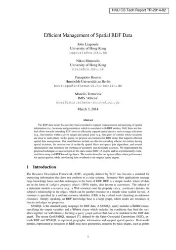
(a)(b)Figure 3: Spatial encoding of entity IDsspatial Filter conditions on-the-fly in a query evaluation plan, and (ii) define spatial operators that applyon the approximations.Figure 3(b) illustrates the Hilbert space filling curve, a classic encoding scheme of spatial locationsinto one-dimensional values. We partition the space using a grid, and order the cells based on the curve.We then divide the ID given to a spatial resource r into two components: (i) the Hilbert order of the cellwhere r spatially resides occupies the m most significant bits (where 2m/2 2m/2 is the resolution of thegrid), and (ii) a local identifier which distinguishes r to other resources that reside in the same cell as r.Since the RDF data may also contain resources or literals, which are not spatial, we use a different rangeof ID values for non-spatial resources with the help of the least significant bit as a flag. In the toy exampleof Figure 3(a), the least significant bit (b0 ) indicates whether the entity modeled by the ID is spatial (b0 1) or non-spatial (b0 0), the next 4 bits are used for the local identifier, and the 6 most significant bitsencode the Hilbert order of the cell. For example, in Figure 3(b), entity e1961 is spatial (b0 is set) and it islocated in the cell with Hilbert order 111101 (cell with ID 61), having local code 0100. For a non-spatialresource, bit b0 would be 0 and the remaining ones would not have any spatial interpretation. Figure 3(c)illustrates which IDs encode the cities of Figure 1(a).In the case of a skewed dataset, a cell may overflow, i.e., there could be too many entities fallinginside it rendering the available bits for the local codes of entities in it insufficient. In this case, entitiesthat do not fit in a full cell are assigned to the parent of the cell in the hierarchical space decomposition.For instance, consider the data in Figure 3(b) and assume than the cell with ID 61 is full and that theentity e1931 cannot be assigned to it. e1931 will be assigned to the parent cell, i.e., the square that consistsof the cells 60, 61, 62, and 63. This cell’s encoding has 4 bits, that is, 2 bits less than its children cells.7

These 2 bits are now used for the local encoding of entities in it. Intuitively, as we go up in the hierarchyof the grid, each cell can accommodate more entities. An entity that must be assigned to an overflowncell ends in the first non-full ascendant of that cell as we go up in the hierarchy. The dlog2 (m/2)e leastsignificant bits of the local code area are reserved to encode the level of the spatially-encoded cell in theID (the most detailed level being 0). In our example, m 6, hence, 2 bits of the local code are used todenote the level of the cell that approximates each entity.The encoding we described is also used for arbitrary geometries that may overlap with more than onecells of the bottom level. For example, the polygon at the lower left corner of the grid of Figure 3(b)spans across cells with IDs 1 and 2, thus, it will be assigned to their parent cell, which has a spatialencoding 0000. Due to the variable number of bits given to the spatial approximations, the encoding isalso suitable for dynamic data (i.e., inserted entities that fall into overflown cells are given less accurateapproximations).The most important benefit of the spatial encoding scheme is that the (approximate) evaluation ofspatial predicates can be seamlessly combined with the evaluation of non-spatial patterns in SPARQL. Forexample, spatial Filter conditions included in a query which are bound to entity variables (for example,?s hasGeometry ?g, Filter WITHIN (?g, “POLYGON(.)”) can be evaluated on-the-fly at any placein the evaluation plan where the entity variable (e.g., ?s) has been instantiated, by decoding the IDsof the instances. Note that the spatial mapping is only approximate (based on the conservative gridapproximation of the spatial locations). Thus, by applying a spatial predicate on the approximations (i.e.,cells) of the entities, false hits may be included in the results, which need to be verified. This is in linewith classic spatial query evaluation approaches [9], which first evaluate all spatial predicates, based onconservative approximations (i.e., MBRs) of spatial objects and then refine the final results by accessingthe exact geometries of the objects. This way, random accesses for retrieving the geometries of entities,whose encoded spatial approximation does not satisfy the spatial Filter conditions of the query can beavoided.A side-benefit of using a Hibert-encoded grid to approximate the object geometries is that by countingthe number of resources in each cell (counting is already performed by the mapping scheme), we can havea spatial histogram to be used for selectivity estimation in query optimization (this issue will be discussedin detail in Section 7). Finally, extending current systems (e.g., RDF-3X) to use this spatial encoding isquite easy.6Query EvaluationWe now show how our encoding scheme further extends the basic framework presented in Section 4to apply spatial filters early and on-the-fly and significantly accelerate the evaluation of GeoSPARQLqueries. In a nutshell, after each non-spatial operator that instantiates entity variables, which also appearin a spatial Filter condition, the condition is applied on the spatially encoded IDs of the entities. Ingeneral, the sooner we apply these on-the-fly spatial filters, the better because they do not incur any I/Ocost and their CPU cost is negligible.3 After the application of a spatial filter, we append a verification bit(or vbit) to the tuples that survive the filter. If, for a tuple, this bit is 1, the tuple is guaranteed to qualifythe corresponding spatial predicate (no verificat

extends the open-source RDF-3X store [22]. RDF-3X encodes all values that appear in SPO triples to identifiers with a help of a dictionary and models the RDF knowledge base as a single, long table of ID triples. A SPARQL query can then be modeled as a multi-way join on the triples table. The system creates a clustered B -tree for each of the six SPO permutations; the query optimizer .