WIXLIB

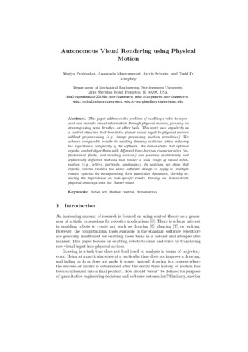
Autonomous Visual Rendering using Physical Motion5FeaturesCFEC E-iSAC PTOFinite Time Horizon Closed Loop Control Nonlinear Dynamics Control Saturation Receding Horizon Continuous Control Weight on Control Efficient Computation Table 1. Comparison of features for the different ergodic control methods used in theexamples.33.1ExamplesWriting SymbolsIn the first example, we investigate how a robot can use ergodic control torecreate a structured visual input, such as a letter, presented as an image. Inaddition, because the input image is not merely of artistic interest but alsocorresponds to a recognizable symbol (in this case, the letter “N”), we showhow a robot can render meaningful visual cues, without the prior knowledge of adictionary or library of symbols. To do this, we represented the image of the letteras a spatial distribution as described in Section 2.1. We then determined thetrajectories for the three different methods (CFEC, E-iSAC, and PTO) describedin Section 2.2 for systems with first order dynamics and second order dynamics.We ran all the simulations for 60 seconds total with the same number of Fouriercoefficients to represent the image spatially.Figure 2 shows the resulting ergodic motions for each control algorithm withthe drawing dynamics represented as a single integrator. From Figure 2, we cansee that while all three methods produce results that are recognizable as the letter“N”, the trajectories generated to achieve this objective are drastically different.The velocity-control characteristic of the single integrator system leads to thesharp, choppy turns evident in both discrete-time CFEC and E-iSAC methods.The infinitesimally small time horizon of the CFEC method, in contrast to thenon-zero receding horizon of the E-iSAC method, results in the large, aggressivemotions of the CFEC result compared to the E-iSAC result. Finally, the weighton the control cost and the continuous-time characteristics of the PTO methodlead to a rendering that most closely resembles typical human penmanship.For the double integrator system shown in Figure 3, the controls are accelerations rather than the velocities of the system. Because of this, the trajectoriesproduced by the discrete controls for the CFEC and E-iSAC method are muchsmoother, without the sharp turns seen in Figure 2. Even though the CFECresult is smoother, its trajectory is more abstract and messy than the singleintegrator trajectory. The receding horizon E-iSAC produces much better results for systems with complicated or free dynamics (e.g., drift), including the

6Autonomous Visual Rendering using Physical MotionCFECE-iSACPTOt10s30s60s10Fig. 2. Trajectories generated by the three different methods with single integratordynamics for the letter “N” at 10 seconds, 30 seconds and 60 seconds with the spatialreconstructions of the time-averaged trajectories generated by each of the methodsat the final time. The different methods lead to stylistic differences with an abstractrepresentation from the CFEC method to a natural, human-penmanship motion fromthe PTO method.double integrator system. The trajectory produced executes an “N” motion reminiscent of human penmanship and continues to draw similarly smooth motionsover the time horizon. While PTO leads to a similarly smooth result comparedto the single integrator system, it leads to a result that less resembles humanpenmanship.From both examples, we can see how ergodicity can be used as a representation of symbolic spatial information (i.e., the letter “N”) and ergodic controlalgorithms can be used to determine the actions needed to sufficiently renderthe information while incorporating the physical capabilities of the robot.Figure 4a-4c shows the ergodic metric, or the difference between the sum ofthe trajectory Fourier coefficients and spatial Fourier coefficients, for the differentmethods over time. We can see that for both dynamic systems, all three methodsproduce trajectories that are similarly ergodic with respect to the letter by theend of the time horizon. Compared to E-iSAC, CFEC converges more slowlywhen more complex dynamics (i.e., double order dynamics) are introduced. PTO

Autonomous Visual Rendering using Physical MotionCFECE-iSAC7PTOt10s30s60sFig. 3. The trajectories generated by the three different methods with double integratordynamics for the letter “N” at 10 seconds, 30 seconds and 60 seconds. The double-orderdynamics lead to much smoother motion from the discrete methods (CFEC and EiSAC) and more ergodic results from the E-iSAC methods due to its receding-horizoncharacteristics.First-order dynamics900.1a.Second-order dynamicsE-iS ACCFECP 0Time (s)b.60400.1Time (s)c.600Time (s)d.60Fig. 4. a)-c) Time evolution of the ergodic metric, or the normalized difference of thesquared sum of the trajectory Fourier coefficients and the spatial Fourier coefficients,for the three different methods with first-order and second-order dynamics for the letter“N” on logarithmic scale. Note that because ergodicity can only be calculated over astate trajectory of finite time duration (see Eq. 1), we start measuring the ergodicityvalues once 0.1 seconds of simulation have passed; hence the three approaches start atdifferent ergodic metrics. All three methods result in similarly ergodic trajectories bythe end of the time horizon, with differences due to their time-horizon characteristics.d) Sum of the Fourier coefficients for the trajectory over time compared to the spatialFourier coefficients of different letters (N, J, L, and M). The trajectory coefficientsconverge to the spatial coefficients of the letter “N” that is being drawn, quantitativelyrepresenting the process of discriminating the specific symbol being drawn over time.exhibits a lower rate of cost reduction because it performs finite-time horizon

8Autonomous Visual Rendering using Physical Motionoptimization. Note that E-iSAC always reaches the lowest ergodic cost value bythe end of the 60 second simulation.Figure 4d compares the sum of the absolute value of the Fourier coefficientstrajectory generated by the CFEC method for the single integrator to the spatial Fourier coefficients of different letters. Initially, the difference between thetrajectory coefficients and spatial Fourier coefficients is large, representing theambiguity of the symbol being drawn. As the symbol becomes more clear, theFourier coefficients of the trajectory converge to the coefficients of “N”, representing the discrimination of the letter being drawn from the other letters.Moreover, letters that are more visually similar to the letter “N” have Fouriercoefficients that are quantitatively closer to the the spatial coefficients of “N”and thus take longer to distinguish which symbol is being drawn. The ergodiccontrol metric allows for representation of a symbol from visual cues and discrimination of that symbol from others without requiring prior knowledge of thesymbols.3.2Drawing ImagesIn the second example, we consider drawing a picture from a photograph asopposed to drawing a symbol. Previously, we were concerned with the representation of the structured symbol. In this example, we move to representing a moreabstract image for purely artistic expression. Here, we are drawing a portrait ofAbraham Lincoln1 with all three methods for single-order and double-order dynamics. We also render the portrait with a lightly damped spring system. Thesimulations are performed for the same 60-second time horizon and number ofcoefficients as the previous example.Figure 5a compares the trajectories resulting from the different ergodic control methods for the single-integrator system. The weight on control and continuoustime characteristics of the PTO method that were desirable for the structuredsymbol example are disadvantageous in this case. While it reduces the ergodiccost, its susceptibility to local minima and its weight on energy lead to a far lessergodic result compared to the other methods.Instead, the discrete nature of the other two methods produce trajectoriesthat are more clearly portraits of Lincoln and are more ergodic with respect tothe photo. The trajectory produced by the CFEC method initially covers muchof the area of the face, but returns to the regions of high interest such thatthe final image produced matches the original image closely in shading. The EiSAC method produces a trajectory that is much cleaner and does not cover theregions that are not shaded in (i.e., the forehead, cheeks). The velocity controlof the single-order system leads to a disjointed trajectory similar to the resultsfrom Fig. 2.Figure 5b compares the resulting trajectories for the double integrator system. As discussed previously, the PTO method produces a trajectory that is far1The image was obtained from https://commons.wikimedia.org/wiki/File:Abraham Lincoln head on shoulders photo portrait.jpg.

Autonomous Visual Rendering using Physical Motion9Fig. 5. Trajectories generated by the three different methods for drawing the portraitof Abraham Lincoln at 10 seconds, 30 seconds and 60 seconds. a) Single IntegratorDynamics: CFEC and E-iSAC result in distinguishable results with stylistic differences,whereas PTO is inadequate for this purpose. b) Double Integrator Dynamics: E-iSACresults in a smooth, clear portrait of Abraham Lincoln with a trajectory that naturallydraws the face as a person would sketch one, without any preprogramming or libraryof motion primitives.less ergodic with respect to the photo. The control on acceleration significantlyimpacts the stylistic rendering of the CFEC rendering. The E-iSAC method produced better results than the other methods for the double integrator system,due to its longer time horizon. The resulting trajectory is smoother and morenatural compared to the single integrator results. Interestingly, this method creates a trajectory that naturally draws the contours of the face— the oval shapeand the lines for the brows and nose— before filling in the details, similar to theway that humans sketch a face [11].Fig. 6 compares the results of ergodicity with respect to time for the differentmethods. Similar to the symbolic example in Section 3.1, the E-iSAC trajectorycreates a more ergodic image by the end for both cases. While the CFEC methodresults in a less ergodic trajectory for both systems, the ergodic cost for thesingle-order dynamics decreases faster for much of the time horizon. The CFECmethod performs significantly worse for the double-order dynamics system andhas a higher ergodic cost than the E-iSAC method throughout the entire timehorizon. The inadequacy of the PTO method for this image is demonstratedhere, having significantly higher ergodic costs at the final time for both systems.Figure 7a compares the renderings of six different images with differentcontent— portraits and monuments using the E-iSAC method with double-orderdynamics. We show that E-iSAC successfully renders different images using asingle set of parameters.

10Autonomous Visual Rendering using Physical MotionSingle-order dynamicsDouble-order dynamicsErgodicity100E-iS ACCFECP TO100ErgodicityE-iS ACCFECP TO1010a.0.1Time (s)b.600.1Time (s)c.60Fig. 6. Time evolution of the ergodic metric, or the normalized difference of the squaredsum of the trajectory Fourier coefficients and the spatial Fourier coefficients for thethree different methods with single-order and double-order dynamics for the Lincolnimage on logarithmic scale. E-iSAC results in a more optimally ergodic trajectory forboth systems. PTO performs poorly for both systems and CFEC performs significantlyworse with the double-order dynamics.a)b)Fig. 7. a) Renderings of different images (Eiffel tower, Marilyn Monroe, Einstein’s face,Lincoln’s face, Einstein with suit, and Taj Mahal) from the double-order dynamicalsystem using the E-iSAC method with the same set of parameters. E-iSAC is ableto successfully render different images with different content (faces and monuments)with the identical parameters. b) Trajectory generated by the E-iSAC method for theLincoln portrait image with damped spring dynamics. E-iSAC is able to produce atrajectory that reproduces the image while satisfying the dynamics of a system.Finally, we demonstrate the ability of the E-iSAC method to take into account more complicated dynamics of the system. In Figure 7b, we simulate asystem where the drawing mass is connected via a lightly damped spring to thecontrolled mass. The resulting Lincoln trajectory is harder to distinguish thanthe renderings from the single-order and double-order dynamical systems. However, the system is successfully able to optimize with respect to the dynamics and

Autonomous Visual Rendering using Physical Motion11draw the main features of the face—the hair, the beard, and the eyes—withinthe time horizon, reducing the ergodic cost by 31.5% in 60 seconds.3.3Comparisons with Existing Robot Drawing TechniquesExisting drawing robots employ a multistage process, using preprocessing (e.g.,edge detection and/or other image processing techniques) and postprocessing(e.g., motion primitives, shade rendering, path planning) to render the image[3, 4, 5, 12, 19]. To accomplish this, most robots and their software are codesigned specifically with drawing in mind, with most specializing in recreatingscenes of specific structures, such as portraits of human faces. Similar multistage methods are commonly used for robot writing. They typically use imagepreprocessing, segmentation, waypoints, or a library of motion primitives toplan the trajectory and execute the trajectory using different motion controland trajectory tracking methods [9, 16, 18, 22].a) Edge Detectionb) Paul the Robotc) Ergodic ControlFig. 8. Comparison of Drawing Methods. a) Edge detection and Binarization methodused in [3] b) Method used by Paul the Drawing Robot from [19] and c) Ergodic Control.Ergodic Control is able to achieve comparable results with an algorithm requiring fewerindependent processes.Recently, some approaches using motion-driven machine learning have beenused to enable robots to learn and mimic human motion [10, 18, 21]. Thesemethods can be difficult and computationally costly and efforts to make themtractable (i.e., predefined dictionary of symbols) can be limiting in scope [9, 22].

12Autonomous Visual Rendering using Physical MotionFurthermore, they do not consider the robot’s physical capabilities and can thusgenerate motions that are difficult for the robot to execute.a)b)Original ImageEdge Detection RenderingE-iSAC Renderinga)Original ImageEdge Detection PreviewE-iSAC RenderingFig. 9. Comparison of the method in [3] and the E-iSAC method. a) The original image and edge detection rendering using the HOAP2 robotic system come directly from[3]. While the edge detection method is successful, producing a tractable trajectoryrequires morphological filters to extract the facial features and predetermined drawingprimitives to render the shading. b) Comparison for a landscape image, with a preview of the overlaid edge detection and binarization results compared to the E-iSACtrajectory. Producing a motion trajectory from the extracted contours of the previewwould be computationally difficult (over 22000 contours result from the edge detection)or needs content-specific postprocessing, and requires a precise drawing system. TheE-iSAC rendering results in a highly tractable result.For comparison, we contrast ergodic control to the method employed in [3],a multi-stage process described in Figure 8a, with a preliminary stage to renderthe outlines of the important features using edge detction and a secondary stageto render shading using image binarization. Figure 9a shows the results of themethod from [3] compared to the trajectory created using the E-iSAC methodfor the double-order system. While the edge detection method from [3] rendersa successful recreation, obtaining a tractable trajectory requires parameter tuning and filtering to extract the most important features from the drawing, andpredetermined drawing primitives and postprocessing to formulate the planartrajectory needed for rendering. Furthermore, the E-iSAC method is able tocapture different levels of shading as opposed to the method in [3] that onlyrenders a binary image (black and white).In addition, because the processing (e.g., filtering, parameter tuning) usedby [3] is tailored to drawing human portraits, the method is not robust to othercontent. To show this, we compare the results for rendering a landscape in Figure9b. While the simulated preview of the rendering appears successful, the image

Autonomous Visual Rendering using Physical Motion13binarization to render shading fails as it is tuned specifically for human portraits.Instead, the quality of the image comes entirely from the edge detection step.However, processing and rendering the contours would be difficult (over 22,000contours are generated to render the image), and the filtering implemented tomake the results tractable are tailored specifically for facial portraits. While theE-iSAC method results in a more abstract image, the trajectory produced istractable and the method is robust to a variety of subjects (as shown in Figure7a).Original ImageRendering with Visual Feedback Rendering with Comp. FeedbackOriginal ReconstructionVisual Feedback ReconstructionComp. Feedback ReconstructionE-iSAC Reconstruction233.5Rendering with E-iSAC21.5Ergodic Cost:0.01.5.7995.120.22.700.6Fig. 10. Comparison of drawings rendered with Paul the Robot [19] and the drawingrendered with E-iSAC and the ergodic Fourier reconstructions of these results. Theoriginal image and the images of the renderings from feedback come directly from [19].The E-iSAC rendering is able to perform comparably to the visual-feedback rendering(a closed-loop algorithm) and better than the computational-feedback rendering (anopen-loop algorithm) with a simpler, open-loop algorithm. The reconstructions of theFourier coefficients representing the different renderings with the respective ergodiccosts show how ergodicity can be used as a quantitative metric for assessment of results.Another drawing method is performed by Paul the robot [19], which uses acomplicated multi-stage process (shown in Figure 8b) to render portraits. Thefirst stage involves a salient-line extraction to draw the important features, andthen performs a shading method using either visual feedback or computationalfeedback. The visual-feedback shading process uses an external camera to update the belief in real-time, while the computational-feedback shading process isbased on the simulation of the line-extraction stage and is an open-loop process,similar to the E-iSAC method. Figure 10 compares the results of Paul the robot[19] with the E-iSAC method, and shows the reconstructions of the Fourier coefficients representing each rendering. While the robot successfully renders theimage, the E-iSAC method performs comparably well with a much simpler, openloop algorithm and could be improved with the integration of an external camerasetup to update the drawing in real-time. Furthermore, the method from [19]relies on a highly engineered system that moves precisely and cannot take intoaccount a change in the robotic system, unlike E-iSAC. In addition, Figure 10

14Autonomous Visual Rendering using Physical Motionshows the reconstructions of the Fourier representing each rendering, demonstrating how e

Autonomous Visual Rendering using Physical Motion 3 2 Methods 2.1 Ergodicity Ergodicity compares the spatial statistics of a trajectory to the spatial statistics of a desired spatial distribution. A trajectory is ergodic with respect to a spatial distribution if the time spent in a region is