Transcription
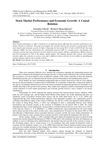
IOSR Journal of Business and Management (IOSR-JBM)e-ISSN: 2278-487X, p-ISSN: 2319-7668. Volume 22, Issue 7. Ser. VII (July 2020), PP 09-21www.iosrjournals.orgStock Market Performance and Economic Growth: A CausalRelationAnindita Ghosh1, RishavChhaochhoria21Assistant Professor in Economics, Department of Commerce,St. Xavier’s College (Autonomous), Kolkata, 30, Park Street, Kolkata- 700016 West Bengal, India2Student (Third Year), Department of Commerce, St. Xavier’s College (Autonomous), Kolkata30, Park Street, Kolkata- 700016West Bengal, IndiaAbstractStock market performance is often considered as an important factor affecting the economic performance of anation, directly or indirectly. This paper investigates the causality between the activities or performance of thestock market and economic growth in India. Using data for the period 2011-12 Q1 to 2019-20 Q3, the studyemployed ARDL Test for determining the relationship between GDP at constant prices representing realeconomic activity and some measures of stock market activity namely: Market capitalisation, Market turnoverand Net Investments by FIIs in the Indian capital market. The findings indicate that various stock marketactivities affect the economy in various ways and to different extents and they do not exhibit an unambiguouspositive relation with the real economic activity.Key Words: Stock Market, Economic Growth, ARDL ----------------------------------------- e of Submission: 05-07-2020Date of Acceptance: ---------------------------------------------I. IntroductionThere exist extremely different views amongst the economists regarding the relationship between thephenomenon of financial development and economic growth, as being clearly indicated in the existing literature.The occurrences of several financial crises in different countries of the world, especially in their post financialliberalisation periods, give an indication that the finance growth relationship is not unambiguously positive.Stock markets are some institutional arrangements that are closely observed not only by every industrybut also by the government of a nation and its Central Bank. It is sometimes evident that a rising stock market isthe sign of a developing industrial sector, but it has always remained an interesting question for researchers as towhether they help in the growth of the economy. Most studies have depicted a positive relationship between thevarious indicators of stock market performance and economic growth; however, such a relation is not alwaysunambiguous.Gadasandula, K. (2019) analysed the relation between four macroeconomic factors; Inflation, GDP,bank rate and exchange rate, and the Indian Stock Market (Nifty Index), the results indicating that there aresignificant causal associations between those factors and the Nifty Index.Nazir, M. S., et al. (2010) alsosuggested that the stock market performance indicators (four dependent variables) were significantly positivecorrelated with GDP per capita, in the context of Pakistan. Ho, Sin-Yu. (2018) also depicted similar findings inthe context of Hong Kong. Petros, J. (2011) has attempted to show a relationship between stock marketdevelopment and economic growth, in the economy of Zimbabwe for the period 1991 to 2007, the resultsindicating that there existed significantly strong positive correlation between the two in the short run as well asin the long run. Gürsoy, C. T. & Müslümov, A. (2000) examined the causal relationbetween the stock marketand economic growth in the context of time series data summarized for 20 nations for the period 1981 to 1994and indicated a bidirectional causal association between economic growth and stock market performance ofnations in the long run, and a causation from economic growth to stock market development in the short run.On the contrary, Singh, A. (1997) concludes that stock market development has been essential for bothinternal and external financial liberalization in 1980s to 1990s and is still continuing, but these developments areunlikely to assist in obtaining faster industrialization and quicker long term growth of the economy in many ofthe developing nations, due to varied reasons; it is not mandatory that stock market development results ineconomic growth. Similarly, Jarrett, J. E., et al. (2009) depicts that the Chinese financial market returns and theprices are not a reliable barometer of the changes in the country’s economy and there is no proof that the SZ andthe SH Granger cause economic prosperity in China.Like any other financial market, stock markets operate through the channels of financialintermediation, diverting savings efficiently into productive investment opportunities. They ensure liquidity atDOI: 10.9790/487X-2207070921www.iosrjournals.org9 Page
Stock Market Performance and Economic Growth: A Causal Relationthe same time providing avenues for higher returns, risk diversification, faster trading of stocks and huge marketof resources for corporates. Thus, financial markets are expected to enhance business activities and canbepositively correlated with economic growth in a country.Caporale, G. M., et al. (2005), revisits therelationship between stock market development and economic growth by forming a theoretical basis to establishthe channels by which these markets affect long run growth of the economy, and the findings indicates thatthrough the channel of investment productivity, growth and development of the economy can be pushed up byshare markets in less-developed countries in the long run. The results of Agarwal, S. (2001)showed thatdevelopment in stock market development and investment are very much interrelated and in turn the former islinked with economic growth.Higher returns and greater access to liquidity however, can bring down precautionary savings as thesemight seem more lucrative to the risk-taking investors. Also, interest rates may rise too high due to theincidence of huge volatility in stock market prices which may lead to inefficient resource allocation and greaterunpredictability, thus resulting in compromises with the productive capacity as well as the quantity ofinvestment thereby hindering economic growth. Nazir, M. S., et al. (2010) indicates that the size of the stockmarket is seen to depict a stronger positive relation or influence than liquidity on growth.The Efficient Market Hypothesis suggests that an efficient capital market enables the prices of thesecurities to rapidly adjust by accommodating to any new information that is available.Hence, the current periodprices of the securities should reflect all available information about the various aspects of the securities. It is inthis context that it can be stated that movements or changes in stock prices should reflect future expectationscorporate performance and corporate profits. If stock prices are effective in accurately reflecting the underlyingfundamentals, then they can be used as leading indicators of future economic activities and economic growth,highlighting the causality between the macroeconomic variables and stock prices and its importance in policymaking. However, Singh, D. (2010) showed that the prices in the Indian Stock Market did not alwaysincorporate all the available information and thus not all macroeconomic variables cannot be used as a tradingtool to earn supernormal profits in the nascent stock market of India. There exists “informational inefficiency”in the several markets influencing macroeconomic variables like WPI, exchange rate, etc. Mohtadi, H. &Agarwal, S. (2007), showed that in the long run an economy’s growth and the stock market are related to oneanother positively; however, the value of share traded ratio is not a correct barometer of stock market liquiditybecause developing countries experience high volatility in their markets causing mispricing of shares.With the end of 2019, there were various market experts in India who had raised the doubt regardingthe stability of the bullish market stressing on the fact that this bullish trend indicated an apparent disconnect thestock market performance and the harsh economic realities faced by the country. The macroeconomic scenarioindicated that India’s GDP growth had declined sharply to six-year lows during the quarters of April-June andJuly-September of 2019-20, owing primarily to a fall in consumption demand. On the other hand, the Sensextouched the 41,000 mark for the first time ever and the Nifty surpassed the 12,100 mark. This situation in thecontext of the Indian economy indicated that the performance of stock markets and the macroeconomicperformance can often change in opposite directions due to the fact that the investors and hence the financialmarkets are often affected by global developments and global fund flows. Moreover, it is alsothe fact that theinvestors and the markets are forward looking so that anyunfavourable news tends to get discounted veryquickly in the markets, thus shifting the focus of governments and companies towards remedial actions. Allthese get reflected in the stock prices, often creating an unambiguous relation or a puzzle for the people who areoutside the market ecosystem.An opposite event was seen to happen during the year 2015-16, when the Indian economy grew atnearly 8 per cent, witnessing the highest rate of growth during the recent years and also during the entire decade,the stock markets performed terribly. The Sensex and the declined sharply moving into the bear territory in2015, recording declines of 22.92 per cent and 21.99 per cent respectively by February, 2016. These eventsshow that the idea of the stock market performance affecting economic growth of an economy seems to be asufficiently debatable issue.This paper attempts to examine the effect of stock market development on economic growth in thecontext of the Indian economy. Our results did not fully support the general notion of stock market developmentrepresenting the economic condition of India. The stock market represents a vital part of our economic systembut trends in markets cannot be treated as a basis for commenting on the economic condition of India.DOI: 10.9790/487X-2207070921www.iosrjournals.org10 Page
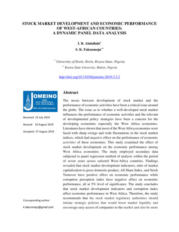
Stock Market Performance and Economic Growth: A Causal RelationII. ObjectiveThe objective ofthe paper is to analyse and understand the effectof stock market activities upon realeconomic activity in the context of the Indian economy. GDP at Constant Pricesis considered to represent realeconomic activity and stock market activities are indicated by the variables - Market Capitalisation; MarketTurnover and Net Investments made by Foreign Institutional Investors (FIIs) in the Indian Capital Market.AnalysisForthe analysis, an attempt has been made to find out the effect of changes in the selected stock marketvariables upon the variable GDP at Constant Prices, representing economic growth. The data on the selectedvariables are collected from the websites of the Central Statistical Organisation and the Reserve Bank of India,indicating that secondary data has been used for the analysis. The same has been attached in Annexure-1. Timeseries data have been taken on all these variables consisting of 35 time periods (or quarters) starting fromQuarter 1 of the Financial Year 2011-12 to Quarter 3 of Financial Year 2019-20.The variables considered for the purpose of analysis are explained here: GDP at constant pricesis also referred to as Real GDP and is calculated by taking into considerationthe prices of some base year, thus adjusting for any price changes or inflation happening between the currentyear and the base year. Hence, GDP at Constant Prices represents the real economic activity; Market Capitalisation of BSE and NSE together refers to the sum total of all the shares listed for allthe public enterprises that are traded on these exchanges multiplied with their respective share prices; Market Turnover of BSE and NSE together, for a time period, is calculated as the ratio of the totalnumber of shares that were traded on these exchanges by the mean number of shares listed on the BSE and theNSE. It represents the liquidity prevailing in the market; Net Investments by FIIs into our country’s capital markets refers to the difference between theinvestments made by foreign institutions in our stock market and the investments made by Indian institutions inforeign capital markets. Institutional Investors includes the likes of mutual funds, hedge funds, insurancecompanies etc.Toconduct a Time Series Analysis, the first requirement is to check whether the time series variables arestationary or not i.e. whether they have a unit root or not. A time series analysis of the variables can beconducted only when all the variables are made stationary, i.e., there should not exist any trend for any of thevariables, i.e., there should be no presence of unit root.A time series data is said to be stationery if the mean and the variances of the variables remain constant overtime.Also, the covariance depends on the time lag between two values of a variable, and not on the specific timeperiods chosen.The Eviews software has been used for the analysis of the data.Graph 1: Graphical Representation of the time series of GDP at Constant PricesGDP at Constant 02,000,0005101520253035Graph 1 gives a clear indication that there is an increasing trend in the time series data of GDP at ConstantPrices. However, to have a confirmation of the presence of trend in the data, the ADF test is conducted, theresults of which are presented below.DOI: 10.9790/487X-2207070921www.iosrjournals.org11 Page
Stock Market Performance and Economic Growth: A Causal RelationTable 1: Augmented Dickey-Fuller Unit Root Test of GDP at Constant PricesNull Hypothes is : GDP AT CONSTANT PRICES has a unit rootExogenous : Cons tant, Linear TrendLag Length: 4 (Automatic - bas ed on AIC, maxlag 8)Augmented Dickey-Fuller tes t s tatis ticTes t critical values :1% level5% level10% levelt-Statis 4*MacKinnon (1996) one-sided p-values .Augmented Dickey-Fuller Tes t EquationDependent Variable: D(GDP AT CONSTANT PRICES)Method: Leas t SquaresDate: 04/01/20 Time: 20:39Sample (adjus ted): 6 35Included obs ervations : 30 after adjus tmentsVariableCoefficientStd. Errort-Statis ticGDP AT CONSTANT PRICES(-1)D(GDP AT CONSTANT PRICES(-1.D(GDP AT CONSTANT PRICES(-2.D(GDP AT CONSTANT PRICES(-3.D(GDP AT CONSTANT squaredAdjus ted R-squaredS.E. of regres s ionSum s quared res idLog likelihoodF-statis ticProb(F-statis tic)0.9413560.92605826282.281.59E 10-343.882161.533070.000000Mean dependent varS.D. dependent varAkaike info criterionSchwarz criterionHannan-Quinn criter.Durbin-Wats on s ble 1 represents the results of the ADF test conducted on the time series data of GDP at ConstantPrice (at levels). The t-statistic value (2.207818) of the ADF test indicates that its absolute value is less than thecritical value(s) (particularly the critical value at the 5% level of significance) and the associated probability ofthis t-statistic value is much greater 0.05 (0.4684). These results indicate that the null hypothesis of the ADF testis accepted i.e., the time series data of GDP at Constant Prices has a unit root (the time series is non-stationary).Moreover, the second part of the table shows that the trend coefficient (18746.97) is statistically significant andmuch greater than 1. All these observations imply that the data is not stationary.To undertake time series analysis, the non-stationarity should be removed and for this the first difference of thedata on GDP at Constant Prices is considered, and again the ADF test is conducted.Table 2 : Augmented Dickey-Fuller Unit Root Test of First Difference of GDP at Constant PricesNull Hypothesis: D(GDP AT CONSTANT PRICES) has a unit rootExogenous: Constant, Linear TrendLag Length: 3 (Automatic - based on AIC, maxlag 8)Augmented Dickey-Fuller test statisticTest critical values:1% level5% level10% 3.2183820.4924*MacKinnon (1996) one-sided p-values.DOI: 10.9790/487X-2207070921www.iosrjournals.org12 Page
Stock Market Performance and Economic Growth: A Causal RelationAugmented Dickey-Fuller Test EquationDependent Variable: D(GDP AT CONSTANT PRICES,2)Method: Least SquaresDate: 04/01/20 Time: 20:43Sample (adjusted): 6 35Included observations: 30 after adjustmentsVariableCoefficientStd. Errort-StatisticProb.D(GDP AT CONSTANT PRICES(-1))D(GDP AT CONSTANT PRICES(-1),2)D(GDP AT CONSTANT PRICES(-2),2)D(GDP AT CONSTANT 60.02030.6722R-squaredAdjusted R-squaredS.E. of regressionSum squared residLog 929628324.401.93E 10-346.7654184.10010.000000Mean dependent varS.D. dependent varAkaike info criterionSchwarz criterionHannan-Quinn criter.Durbin-Watson 03Table 2 represents the results of the ADF test on the first differences of the time series data on GDP atConstant Prices. The results reflected in this table can be interpreted in exactly similar way as in the caseofTable 1. Hence, comparing the value of the ADF t-statistic with the critical values, and considering theassociated probability of the ADF t-statistic, we can conclude that the time series data on the first difference ofGDP at Constant Prices is non-stationary (i.e., the null hypothesis of the presence of a unit root is accepted).Moreover, the second part of the table again shows that the trend coefficient (325.4419) is still much greaterthan 1, but not statistically significant.The results of Table 2 indicate that the trend has not been removed through first differencing, and hence weshould consider the second differencing of the data.Table 3: Augmented Dickey-Fuller Unit Root Test of Second Difference of GDP at Constant PricesNull Hypothesis: D(GDP AT CONSTANT PRICES,2) has a unit rootExogenous: Constant, Linear TrendLag Length: 2 (Automatic - based on AIC, maxlag 8)Augmented Dickey-Fuller test statisticTest critical values:1% level5% level10% 3.2183820.0000*MacKinnon (1996) one-sided p-values.Augmented Dickey-Fuller Test EquationDependent Variable: D(GDP AT CONSTANT PRICES,3)Method: Least SquaresDate: 04/01/20 Time: 20:44Sample (adjusted): 6 35Included observations: 30 after adjustmentsDOI: 10.9790/487X-2207070921www.iosrjournals.org13 Page
Stock Market Performance and Economic Growth: A Causal RelationVariableCoefficientStd. Errort-StatisticProb.D(GDP AT CONSTANT PRICES(-1),2)D(GDP AT CONSTANT PRICES(-1),3)D(GDP AT CONSTANT .00000.00000.00000.25960.2931R-squaredAdjusted R-squaredS.E. of regressionSum squared residLog 907530334.272.30E 10-349.4343657.36510.000000Mean dependent varS.D. dependent varAkaike info criterionSchwarz criterionHannan-Quinn criter.Durbin-Watson 98Table 3 represents the results of the ADF test conducted on the second differences of the data on GDPat Constant Prices. The results highlight that the value of the ADF test statistic (36.00838) larger in absolutevalue than the critical value(s) particularly at 5% level of significance. Moreover, the associated probability withthe ADF t-statistic value is less than 0.05, indicating that the null hypothesis is rejected, i.e., there is no presenceof unit root. This implies that the data has now become stationary.Moreover, the second part of the table shows that the trend coefficient (- 657.3651) has become lessthan 1 and the associated probability of (0.2931) indicates that the null hypothesis of the presence of unit root isrejected.Thus, the trend in the data has been removed after take second differences, implying that our timeseries data on GDP at Constant Prices is Integrated of Order 2, i.e., I(2).Graph 2: Graphical Representation of the time series of Market Capitalisation (BSE NSE)Market Capitalisation (BSE aph 2 represents the time series data on Market Capitalisation in BSE and NSE taken together. This graphicalrepresentation indicates that there is not a clear increasing or decreasing trend over time. To confirm thepresence or absence of a trend, we again conduct an ADF test, as shown in the following Table 4.Table 4 : Augmented Dickey-Fuller Unit Root Test of Market Capitalisation (BSE NSE)Null Hypothesis: MARKET CAPITALISATION B has a unit rootExogenous: Constant, Linear TrendLag Length: 3 (Automatic - based on AIC, maxlag 8)Augmented Dickey-Fuller test statisticTest critical values:DOI: 10.9790/487X-22070709211% level5% level10% 4-4.284580-3.562882-3.2152670.014314 Page
Stock Market Performance and Economic Growth: A Causal Relation*MacKinnon (1996) one-sided p-values.Augmented Dickey-Fuller Test EquationDependent Variable: D(MARKET CAPITALISATION B)Method: Least SquaresDate: 04/01/20 Time: 20:53Sample (adjusted): 5 35Included observations: 31 after adjustmentsVariableCoefficientStd. Errort-StatisticProb.MARKET CAPITALISATION B(-1)D(MARKET CAPITALISATION B(-1))D(MARKET CAPITALISATION B(-2))D(MARKET CAPITALISATION R-squaredAdjusted R-squaredS.E. of regressionSum squared residLog 76763037135.2.31E 14-503.37204.1978840.006602Mean dependent varS.D. dependent varAkaike info criterionSchwarz criterionHannan-Quinn criter.Durbin-Watson 39The results of Table 4 represent that the absolute value of the ADF t-statistic (4.130634) is greater thanthe absolute value of the critical value at 5% level of significance (3.562882), and the associated probability ofthe ADF t-statistic (0.0143) is less than 0.05. These findings indicate that the null hypothesis is rejected at the5% level of significance, implying that there is stationarity at this level of significance.However, the second part of this table indicates that the value of the trend coefficient is still positive,but this is significant only at the 1% level of significance.Hence, concentrating on the 5% level of significance, we conclude that the time series data on MarketCapitalisation (BSE NSE) is stationary, i.e., there is no presence of unit root or trend. Thus, this series isintegrated of order zero, i.e., I(0) at the 5% level of significance.Graph 3: Graphical Representation of the time series of Market Turnover (BSE NSE)Market Turnover (BSE ,000,000500,0005101520253035Graph 2 represents the time series data on Market Turnover in BSE and NSE taken together. This graphicalrepresentation also does not indicate clearly the presence of increasing or decreasing trend over time. Toconfirm the presence or absence of a trend, we again conduct an ADF test, as shown in the following Table 5.DOI: 10.9790/487X-2207070921www.iosrjournals.org15 Page
Stock Market Performance and Economic Growth: A Causal RelationTable 5: Augmented Dickey-Fuller Unit Root Test of Market Turnover (BSE NSE)Null Hypothesis: MARKET TURNOVER BSE NSE has a unit rootExogenous: Constant, Linear TrendLag Length: 0 (Automatic - based on AIC, maxlag 8)Augmented Dickey-Fuller test statisticTest critical values:1% level5% level10% 3.2070940.1384*MacKinnon (1996) one-sided p-values.Augmented Dickey-Fuller Test EquationDependent Variable: D(MARKET TURNOVER BSE NSE)Method: Least SquaresDate: 04/01/20 Time: 21:07Sample (adjusted): 2 35Included observations: 34 after adjustmentsVariableCoefficientStd. Errort-StatisticProb.MARKET TURNOVER BSE .04620.0021R-squaredAdjusted R-squaredS.E. of regressionSum squared residLog 1113235405.81.72E 12-467.22185.6840650.007889Mean dependent varS.D. dependent varAkaike info criterionSchwarz criterionHannan-Quinn criter.Durbin-Watson 72Like the previous cases, the results of Table 5 indicate that the null hypothesis is accepted and hencethere is the presence of a unit root i.e., a trend is present in the data at levels. Hence, we consider the firstdifference of the data and again conduct the ADF test.DOI: 10.9790/487X-2207070921www.iosrjournals.org16 Page
Stock Market Performance and Economic Growth: A Causal RelationTable 6: Augmented Dickey-Fuller Unit Root Test for First Difference of Market Turnover (BSE NSE)Null Hypothesis: D(MARKET TURNOVER BSE NSE) has a unit rootExogenous: Constant, Linear TrendLag Length: 7 (Automatic - based on AIC, maxlag 8)Augmented Dickey-Fuller test statisticTest critical values:1% level5% level10% 3.2334560.0254*MacKinnon (1996) one-sided p-values.Augmented Dickey-Fuller Test EquationDependent Variable: D(MARKET TURNOVER BSE NSE,2)Method: Least SquaresDate: 04/01/20 Time: 21:08Sample (adjusted): 10 35Included observations: 26 after adjustmentsVariableCoefficientStd. Errort-StatisticProb.D(MARKET TURNOVER BSE NSE(-1))D(MARKET TURNOVER BSE NSE(-1),.D(MARKET TURNOVER BSE NSE(-2),.D(MARKET TURNOVER BSE NSE(-3),.D(MARKET TURNOVER BSE NSE(-4),.D(MARKET TURNOVER BSE NSE(-5),.D(MARKET TURNOVER BSE NSE(-6),.D(MARKET TURNOVER BSE 00.02690.18180.48640.0239R-squaredAdjusted R-squaredS.E. of regressionSum squared residLog 2665250573.51.00E 12-353.80005.2132400.002091Mean dependent varS.D. dependent varAkaike info criterionSchwarz criterionHannan-Quinn criter.Durbin-Watson 97The results of the ADF test presented in Table 6 indicates that the null hypothesis is rejected at the 5%level of significance because the absolute value of the ADF t-statistic is greater than the absolute critical valueat the 5% level of significance (also the probability associated with the ADF t-statistic is less than 0.05). Hence,the data series at the first differences has become stationary and is said to be integrated of order 1, i.e., I(1) at the5% level of significance.DOI: 10.9790/487X-2207070921www.iosrjournals.org17 Page
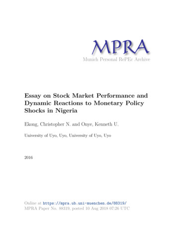
Stock Market Performance and Economic Growth: A Causal RelationGraph 4: Graphical Representation of the time series of Net Investments by FIIs in the Indian CapitalMarketsNet Investments by FIIs in Indian Capital 35Graph 4 gives a clear indication that there is no trend in this time series data on Net Investments by FIIs in theIndian Capital Markets. However, in order to have a confirmation of this stationarity or absence of trend in thedata, we need to conduct the ADF test, the results of which are presented below.Table 7 : Augmented Dickey-Fuller Unit Root Test of Net Investments by FIIs in the Indian CapitalMarketsNull Hypothes is : NET INVESTMENTS BY FIIS has a unit rootExogenous : Cons tant, Linear TrendLag Length: 0 (Autom atic - bas ed on AIC, m axlag 8)Augm ented Dickey-Fuller tes t s tatis ticTes t critical values :1% level5% level10% levelt-Statis 2*MacKinnon (1996) one-s ided p-values .Augm ented Dickey-Fuller Tes t EquationDependent Variable: D(NET INVESTMENTS BY FIIS )Method: Leas t SquaresDate: 04/01/20 Tim e: 21:12Sam ple (adjus ted): 2 35Included obs ervations : 34 after adjus tm entsVariableCoefficientStd. Errort-Statis ticNET INVESTMENTS BY FIIS 9116.860410.3368-5.7651062.723862-1.128754R-s quaredAdjus ted R-s quaredS.E. of regres s ionSum s quared res idLog likelihoodF-s tatis ticProb(F-s tatis tic)0.5174700.48633922943.961.63E 10-388.061116.622370.000012Mean dependent varS.D. dependent varAkaike info criterionSchwarz criterionHannan-Quinn criter.Durbin-Wats on s 23.1382723.049521.983203The results of the ADF test presented in Table 7 indicates that absolute value of the ADF t-statistic(5.765106) is greater than the absolute critical values, and the associated probability is less than 0.05 (0.0002).Moreover, the second part of the table indicates that the trend coefficient is significantly less than 1. Theseresults imply that the series is stationary that is there is no unit r
bank rate and exchange rate, and the Indian Stock Market (Nifty Index), the results indicating that there are significant causal associations between those factors and the Nifty Index.Nazir, M. S., et al. (2010) also suggested that the stock market performance indicators (four dependent variables) were significantly positive