Transcription
Rebound EffectsPrepared for the New Palgrave Dictionary of EconomicsKenneth GillinghamYale UniversityNovember 11, 2014AbstractIn environmental and energy economics, rebound effects may influence the energy savings fromimprovements in energy efficiency. When the energy efficiency of a product or serviceimproves, it becomes less expensive to use, income is freed-up for use on other goods andservices, markets re-equilibrate, and there may even be induced innovation. These effectstypically reduce the direct energy savings from energy efficiency improvements, but lead toimproved social welfare as long as there are not sufficiently large externality costs. There isstrong empirical evidence that rebound effects exist, yet estimates of the different effects rangewidely depending on context and location.KeywordsEnergy efficiency; climate policy; take-back effect; backfire; emissions; welfare; greenhousegases; derived demand1
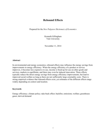
IntroductionEnergy efficiency policies are among the most common environmental policies around theworld. Holding consumer, producer, and market responses constant, an increase in energyefficiency for an energy-using durable good, such as a vehicle or refrigerator, willunambiguously save energy. Rebound effects are consumer, producer, and market responses toan increase in energy efficiency that typically reduce the energy savings that would haveoccurred had these responses been held constant. The use of the term “rebound” is intuitive: theresponses lead to a rebounding of energy use back towards the energy use prior to the energyefficiency improvement. For this reason rebound effects are sometimes also called “take-back”effects, for some of the energy savings are “taken-back” by the responses.Often rebound effects are referred to in the singular, as “the rebound effect,” but it is widelyunderstood that there are actually several effects at work. At one extreme, these rebound effectscan lead to additional energy use above the amount used prior to the energy efficiencyimprovement. This is often called “backfire,” referring to the energy efficiency improvement“backfiring” in terms of saving energy. At the other extreme, negative rebound effects, wherebythe responses increase the energy savings, are may be possible as well. In economics, reboundeffects most often are in reference to energy use, but of course rebound effects can also bedescribed in terms of greenhouse gas emissions or other measures of environmental impact.Moreover, rebound effects are possible in other areas as well, such as materials or water. Thisarticle follows the convention and focuses on rebound effects in energy use.Figure 1 illustrates the importance of rebound effects for the energy savings that can be expectedfrom the 2017-2025 Corporate Average Fuel Economy Standards in the United States. Thisillustration assumes a 30 percent total rebound effect, which would “take-back” 0.30 quadrillionBTU of the energy savings that would have been expected from the policy.2
Figure 1. 2025 US transport sector energy use with the 2017-2025 CAFE standards illustrating how rebound effects mayinfluence energy savings (Gillingham et al., 2013). The figure assumes a 30% rebound effect for illustrative purposes.The first mention of rebound effects goes back to the English economist William Stanley Jevonsin 1865. Jevons lived at a time when coal-fired steam engine technology was dramaticallyimproving in England. Yet, despite improvements in engine efficiency, coal use was notdeclining, but rather was increasing. Jevons attributed this to the improved productivity of coaluse, leading to more investment and growth in the sectors of the economy that used coal. Jevonsfamously stated “It is a confusion of ideas to suppose that the economical use of fuel isequivalent to diminished consumption. The very contrary is the truth” (Jevons, 1865). Thebackfire that Jevons was positing has more recently been called the “Jevons Paradox,” for itseems paradoxical to have an energy efficiency improvement lead to more energy use.More recently, policymakers and academics have been increasingly interested in rebound effectsfrom energy efficiency policies. If there are large rebound effects leading to backfire, energyefficiency policies may not save energy at all. Moreover, larger rebound effects would beexpected to widen the welfare difference between first-best policies to address market failures,such as price policies to correct for externalities, and energy efficiency policies, which aregenerally considered second-best policies (unless there are behavioral failures, as described inGillingham and Palmer (2014) and many other papers). Such observations have led to a vibrantacademic and policy debate over the magnitude of the effects.Rebound effects are often broadly classified into their microeconomic and macroeconomiceffects. We proceed by discussing each and then turn to quantification and policy implications.Microeconomic Rebound Effects3
The microeconomic rebound effect may occur for both consumers and firms when there is anenergy efficiency improvement. Most of the economic literature focuses on consumers, so webegin here with the microeconomic rebound effect from the consumer perspective.The microeconomic rebound effect for consumers captures the change in the consumptionbundle of all goods and services when there is an energy efficiency improvement in one product.For consumers, it stems from the classic substitution and income effects of a price change, as inthe Slutsky equation (Gillingham et al., 2015). Unfortunately, the literature is inconsistent in theterminology used, so it is instructive to begin with some simple microeconomic theory. Thefollowing exposition loosely follows Borenstein (2015).Suppose we have an energy efficiency improvement in an energy-using good 0. For instance, thiscould be a vehicle, light, or air conditioner. Let the original energy intensity (i.e., the reciprocalof energy efficiency) of the good be and the new energy intensity be . With greater energyefficiency, the cost or price of using good 0 drops (i.e., the energy cost of the energy servicedrops). Denote the price of using good 0 as and the change in price with the efficiencyimprovement as Δ . Similarly let the demand for good 0 be . At the same time that the pricedecreases, there may also be a cost ( ) associated with the energy efficiency improvement.The combination of such a price decline and change in income leads to a consumer response infour ways as they re-optimize their consumption bundle.First, there is a substitution effect, whereby the consumer substitutes from other goods andservices to good 0 along the Hicksian (compensated) demand curve of the use of good 0. Theamount of increased consumption is just the marginal change in the Hicksian demand with aprice change () times the change in the price of usage Δ . The increased consumption ofcourse uses energy. The change in energy use from the substitution effect is the new energyintensity of the good times the increased consumption:Δ .Second, there is an income effect. Since the consumer is no longer spending as much on usinggood 0, the consumer may have income to re-spend ( Δ ). For example, if a consumer is nowspending less to drive a mile, they have increased purchasing power. However, the energy. Thisefficiency improvement may come with a cost, so the total change in income is Δchange of income may be positive or negative depending on how costly the efficiencyimprovement is. Furthermore, it can be expected to influence the demand for using good 0. Letthe demand for using good 0 be given by and income be given by I, so the marginal change indemand with a change in income is . Thus, the change in demand for using good 0 with theenergy efficiency improvement is given bythe income effect is thenΔΔand the change in energy use due to.Third, there may be a substitution effect for every other good and service. For goods that aresubstitutes for good 0, there would be a decrease in consumption with a price decrease of good 0.For complements, the opposite. Let the Hicksian (compensated) demand for good be given by4
, and the marginal change in Hicksian demand for good with a change inbe given by.Then, for any good , the change in energy use from the energy efficiency improvement in good0 isΔ , whereis the energy intensity of good (i.e., the amount of energy used inproviding the energy service). Thus the aggregate change in consumption for all other goodsbesides good 0 is Δ . Since some goods are substitutes and others are complements,and goods differ in energy intensity, the sign of this term is ambiguous (Chan and Gillingham,2014, Borenstein, 2015, Berkhout et al., 2000). In general, one might expect it to be negative, forthere is a general substitution in consumption towards good 0 when its efficiency increases.Fourth, there may be an income effect for every other good and service. If there is additionalincome freed-up from the energy efficiency improvement, it can be re-spent on other goods andservices as the consumer re-optimizes consumption. As mentioned above, the change in income. Thus the change inassociated with the energy efficiency improvement is Δconsumption for any good when good 0 has an energy efficiency improvement is simply themarginal change in demand of good with a change in income ( ) times the change in income:Δ. The change in energy use for good is thenΔ, and theaggregate change in energy use for all goods besides good 0 is Δ. The signof this income rebound effect is ambiguous as well. It depends on the change in income, as wellas the relative energy intensity of normal goods versus inferior goods. If nearly all goods arenormal goods and the change in income is positive, one would expect a positive sign for thiseffect.The sum of these four responses forms the basis of the microeconomic rebound effect, whichquantifies the change in energy use with a change in energy efficiency:ΔΔΔΔ.The first two terms (substitution and income effects for good 0) are nearly always defined as thedirect rebound effect, for they capture the direct consumer response in good 0 to the energyefficiency improvement (Sorrell and Dimitropoulos, 2008). Assuming a positive change inincome and usage of good 0 being a normal good, one would expect a positive sign for the directrebound effect.However, the other terms are defined in various ways in the literature, potentially leading toconfusion (Turner, 2013). In particular, the indirect rebound effect is a term widely used in theliterature, yet its usage is inconsistent (Azevedo, 2014, Gillingham et al., 2015). Its nameindicates the more indirect nature by which energy savings are reduced. Many studies refer to theindirect rebound effect as the sum of terms three and four (Chan and Gillingham, 2014). Otherstudies recognize that the indirect rebound effect includes both terms, but focus on onlyestimating the income effect on other goods and services (the fourth term) as a measure of therebound effect (Chitnis et al., 2014). Others simply define the indirect rebound as the fourth term5
(Borenstein, 2015). Still others either explicitly or implicitly use a much broader definition forthe indirect rebound, which includes both the third and fourth terms as well as additional reboundeffects.One of these additional rebound effects is the embodied energy rebound effect, which capturesthe energy used to create the energy efficiency improvement. The sign of this effect is contextdependent. A more energy efficient product may take more or less energy to produce. If theprocess of building a more efficient product is more energy intensive, then the embodied energyrebound would be expected to be positive. Of course, there may be energy embodied in othergoods and services as well, so a broader definition of the embodied energy rebound wouldinclude the change in energy use from embodied energy from other goods and services as well.It is common to include the embodied energy rebound as part of the indirect rebound effect. Forexample, Azevedo (2014) and Thomas and Azevedo (2013b) define the indirect rebound effectas the sum of terms three and four above, and use an energy intensity that includes theembodied energy in both good 0 and all other goods and services. Sorrell (2007) defines the totaleconomywide rebound effect as the sum of the direct and indirect rebound effects. Under thisdefinition, the indirect rebound effect is a residual that includes the third term, fourth term, allembodied energy effects, and macroeconomic rebound effects.Another proposed definition is to call the first three terms in the equation above the “net directrebound effect” for they account for the direct rebound as well as the change in energy use fromall other goods and services, including the ones being substituted away from (Borenstein, 2015).If this third term is negative, we would expect a smaller net direct rebound than direct reboundeffect.For the net energy savings from an energy efficiency improvement (abstracting from anymacroeconomic rebounds), we can compare the microeconomic rebound effect ( ) to the upfrontenergy savings from the efficiency improvement. Thus, the net energy savings after the), minus and minusmicroeconomic rebound would be given by the energy savings,any embodied energy effect ( ):.As mentioned above, the microeconomic rebound effect may also occur for firms. Consider afirm that is using capital and labor to produce a good or service. When there is an energyefficiency improvement, there is a factor-substitution effect: capital becomes relatively moreproductive, so more (energy-using) capital and less (non-energy-using) labor is included in theoptimal production factor mix. Moreover, the marginal cost of production may decline,increasing the optimal amount of production. Both the switch to more energy-using inputs andincrease in production may lead to a rebound effect on the production side (Berkhout et al.,2000). While these production-side rebound effects clearly have microeconomic foundations,nearly all research on them has been at the macroeconomic level, which often aims to take intoaccount the full set of changes in production and prices across the economy.6
Macroeconomic Rebound EffectsThe macroeconomic, or sometimes “economy-wide,” rebound effects involve several channelsby which market responses could influence the energy savings from an energy efficiencyimprovement. There is a macroeconomic price effect or energy market effect, which describeshow a shift inwards in demand for energy in the market due to the energy efficiencyimprovement will be accompanied by a subsequent re-equilibration as prices and quantities areset so that supply equals demand. This market response will mean that the reduction in demandwill be less than the amount that demand is shifted inward. It is governed by the slopes of thesupply and demand curves. The macroeconomic price effect is small if demand is highly elasticand supply is inelastic, for then the market will re-equilibrate at nearly the same quantity as whatyou would have without the re-equilibration process. Similarly, the macroeconomic price effectis large if demand is inelastic and supply is elastic (Borenstein, 2015, Gillingham et al., 2013).This macroeconomic price effect can occur in any market, but is particularly easy to understandwhen there is an energy efficiency improvement shifting demand inward in a single region (e.g.,from a fuel economy standard in the U.S.) and there is a broader market for fuel (e.g., the globaloil market). In the case of oil, the reduced demand for oil in the U.S. leads to a lower global oilprice, and thus induced oil demand elsewhere.Another category of macroeconomic rebound effects can be called the macroeconomic growtheffect, for it describes how the amount of economic growth and patterns of economic growth canbe influenced by the energy efficiency improvement (Gillingham et al., 2013). Jevons was on toa version of this type of rebound effect: a sectoral reallocation rebound effect. Just like thesubstitution effect in consumption, there is analogous effect in investment and production in theeconomy. When the relative rate of return of a sector increases, we would expect to see moreinvestment and economic growth in this sector. Of course, this sectoral general equilibriumeffect depends on two factors: (1) the degree to which the energy efficiency improvementincreases the rate of return of the sector and (2) the energy intensity of production in the sectorrelative to other sectors. The sectoral reallocation rebound could be positive or negative,depending on the cost of the energy efficiency improvement (e.g., is it a mandatory and costlyenergy efficiency increase?) and the energy intensity of the energy-using sector relative to othersectors (e.g., is the shift in production from more energy-intensive or less energy-intensivesectors?). The sectoral reallocation effect can also be extended to a reallocation of innovativeactivity and human capital, such that higher returns in a sector can lead to more innovativeactivity and human capital moving into that sector (Lemoine, 2014).The macroeconomic growth effect may also involve innovation in another way. The process ofresearching to find new ways to improve energy efficiency may engender spillovers to otherprocesses and sectors. For example, finding ultra-lightweight materials for aircraft may spilloverto other manufacturing areas, such as that of electronics or bicycles, spurring economic growth inother sectors. Thus, energy efficiency improvements may change the path of innovation inmultiple areas, leading to broader economic growth.Another possible pathway for a macroeconomic growth effect is through a macroeconomicmultiplier. Macroeconomists have posited that income gains (usually from a government7
program) may have a multiplier effect in times of high unemployment when there is unusedcapacity in the economy (Ramey, 2011). This multiplier effect would occur if a dollar ofadditional income is spent in a way that uses some of the under-utilized labor and capital in theeconomy. Thus, additional income would generate further income and economic growth morebroadly. Of course, this effect may be dampened by any future expected taxes or debt incurred toprovide the income. However, in the context of freed-up income from an energy efficiencyimprovement, the multiplier would not be associated with any additional taxes or governmentdebt, so the effect might be expected to be different (Borenstein, 2015).Other channels may also influence the macroeconomic rebound. For example, Lecca et al. (2014)and Turner (2009) posit an interaction between the macroeconomic price effect and sectoralreallocation, which they call “disinvestment effects.” In the short run, the shift away from energycan lead to excess capacity in energy supply, leading to lower energy prices and thus a greaterrebound. In the longer run, the returns to capital will drop, so this excess capacity will bedivested, which will put upward pressure on energy prices, serving to constrain themacroeconomic rebound. Thus, in contrast to previous theoretical predictions (e.g., Wei (2007)and Saunders (2008)), the macroeconomic rebound may be larger in the short run.Evidence on Rebound Effects: Historical BackgroundThere is an extensive literature aiming to estimate rebound effects in one form or another. Workon the subject ranges from theoretical models with calibrated simulations to empiricalestimations and computable general equilibrium models. Yet the magnitude of the total reboundeffect varies by context and remains controversial. While the literature provides strong guidancefor some microeconomic rebound effects in many contexts, such as the direct rebound effect, it isclear that the relevant magnitude varies by location and setting. The current literature providesless guidance on macroeconomic rebound effects, with different studies capturing differenteffects, and magnitudes ranging from limited rebound to significant backfire.The rebound effect first entered into the modern academic literature in 1979 with Brookes (1979)and Khazzoom (1980), who resurrected the Jevons Paradox in the context of modern energyefficiency policies. In fact, the Jevons Paradox has been referred to as the “Khazzoom-BrookesPostulate” by later studies (Saunders, 1992). Khazzoom (1980) was particularly focused onmicroeconomic rebounds and Brookes (1979) on macroeconomic rebounds, but both posited thatimprovements in energy efficiency may lead to backfire.This view was shortly thereafter critiqued in papers such as Lovins (1988), Henly et al. (1988),and Grubb (1990), which point out that energy demand is relatively inelastic and energytypically is a small percentage of the cost of energy services, so rebound effects for most energyservices might be expected to be small. This led to a series of papers exploring what functionalforms on economy-wide production could lead to backfire when there is an energy efficiencyimprovement. Saunders (1992) assumes a Cobb-Douglas production function, which allowssubstitutability between inputs, and finds that backfire is not only possible, but may even belikely. In contrast, Howarth (1997) assumes an alternative (Leontief) production function whereenergy, labor, and capital are complements, rather than substitutes, and finds that backfire is not8
likely. A take-away from this theoretical literature is that if it is easier to substitute across inputsinto production, then backfire becomes more likely.The first empirical estimates used to describe rebound effects were simply estimates of priceelasticities of demand for energy services, which are taken as a proxy for the direct reboundeffect defined above. Greening et al. (2000) perform a review of the literature estimating priceelasticities of demand for a variety of energy services for both consumers and firms. They findprice elasticities of demand in the wide range of 0 to -0.5, with most studies falling in the rangeof -0.1 to -0.3 (estimates included are both long-run and short-run). This would be interpreted asa direct rebound effect of 0 to 30 percent. Greening et al. (2000) also coined the terms “directeffect,” “indirect effect,” “economy-wide effect,” “transformational effect.” Thetransformational effect had a vague definition relating to changing preferences and has not beencontinued in the subsequent literature. Schipper and Grubb (2000) make perhaps the first roughestimate of the indirect rebound effect, finding that re-spending leads to a 5 to 15 percentrebound. None of the studies estimate the substitution effect on other goods and servicesdescribed above.Since 2000, the literature on rebound effects has grown dramatically and reached beyondeconomics into engineering fields, such as industrial ecology. There are three key strands ofcurrent literature. Most studies on rebound effects estimate a price elasticity of demand for anenergy service, call this the direct rebound effect, and stop there. But there are a few studiesestimating the indirect rebound effect. In addition, there has been recent work using computablegeneral equilibrium models and econometric simulation models aiming to estimate differentmacroeconomic rebound effects. The next sections discuss each of these three strands ofliterature in turn.Evidence on Rebound Effects: Price Elasticities of DemandThe literature estimating price elasticities of demand for energy services is quite large withperhaps hundreds of papers. Of course, with a literature so vast, current estimates still rangewidely, depending on the energy service, time frame (short-run or long-run), years covered,location, and estimation methodology. Some of the most recent reviews of the literature thatfocus on the rebound effect include Sorrell (2007), Azevedo (2014), and Gillingham et al.(2015). Each of these papers includes a table reviewing the estimates in the literature. Broadly,estimates for the direct rebound effect still tend to be in the range of 0 to 50 percent, just as in theearlier Greening et al. (2000) review. Gillingham et al. (2015) narrows this set further by lookingat only more recent studies for a variety of energy services that the authors believe deal withempirical identification issues in a convincing way; these short-run estimates are in a range of 5to 40 percent, with most studies falling in a range of 5 to 25 percent.Notably, most well-identified estimates of the price elasticity of demand are from developedcountries, with the most common relating to transport in the United States. Sorrell (2007) andothers have suggested that the direct rebound effect in developing countries may be larger sincethe demand for energy services may be far from saturated. Indeed, studies from developingcountries show an even greater range of estimates, including some very large direct reboundeffect estimates (Sorrell, 2007). Gillingham et al. (2015) argue that these should be interpreted9
cautiously and that most of the developing country estimates tend to fall in the same 0 to 50percent range as estimates from developed countries.The studies on price elasticities of demand for energy services that contribute to the ranges ofestimates above tend to use detailed disaggregated data from short time periods. This is usefulfor understanding the price responsiveness during that time period, but says little about theresponsiveness during other time periods. A few studies take a longer-term economic historyperspective. For example, Fouquet and Pearson (2012) uses historical time series data on lightingin the United Kingdom from 1750 to the present and estimates a time-varying price elasticity oflighting demand. The results indicate a price elasticity in the eighteenth and nineteenth centuriesthat was indicative of backfire. After 1900, the elasticity was closer to zero, but still indicated asubstantial responsiveness to price (e.g., in the range of -0.5 to nearly -1).Fouquet (2012) performs a similar analysis for transport in the United Kingdom and also finds adeclining responsiveness to energy service price, with the long-run price elasticity of passengertransport demand changing from -1.5 in 1860 to -0.6 in 2010. While these estimates areindicative of more responsiveness than other recent estimates of the price elasticity of transportdemand from the United States (e.g., Small and van Dender (2007) and Gillingham (2014)), it ispossible that they are consistent; not only is the setting is different (e.g., gasoline and dieselprices are higher in the United Kingdom) and but the time frame of the estimate is different (e.g.,long-term versus short-term or medium-term).Other long-term estimates include Tsao et al. (2010), who find backfire in lighting over severalcenturies and Saunders (2013), who estimates backfire or large rebound in many sectors over thepast four decades. These backfire results are perhaps understood in light of the substantialassumptions involved in the analyses. For example, the estimates in Tsao et al. (2010) are basedon the same Cobb-Douglas functional form from earlier work by Saunders (1992), along withmany other assumptions. Saunders (2013) relies on a translog cost function, but makes otherassumptions that have been critiqued (Gillingham et al., 2015). Another interpretation is thatthese studies are estimating something different than the rest of the literature, such as a longerrun effect that implicitly includes other rebound effects, such as macroeconomic rebound effects.Evidence on Rebound Effects: Estimates from PoliciesRather than estimate price elasticities of demand for energy services, which hold all otherattributes of the product constant and assume a costless increase in energy efficiency, a fewstudies relax these assumptions and analyze the rebound effect from a particular policy ortreatment. Gillingham et al. (2015) name this type of rebound a “Policy-induced improvement”(PII). A perfect example is Davis et al. (2015). This study analyzes an experiment in Mexico thatprovides direct cash payments and subsidized financing to consumers replacing old refrigeratorsand air conditioners. The switch from an old to new appliance is potentially associated with avery large change in attributes, with the new appliances providing a much better energy service.Moreover, there is an income effect from the transfer. The results indicate an extremely largerebound from this policy; for instance, electricity use increases after replacement of the airconditioner and only drops by seven percent after replacement of the refrigerator.10
Other examples of studies that estimate this type of rebound are Davis (2008) and Gillingham(2013). Davis (2008) examines a field experiment where households received free energyefficient clothes washers. Subsequently, they increased washing by 5.6 percent. These clotheswashers were not only more energy efficient, but also were larger and gentler on more clothes, sothis rebound effect estimated is the combined effect of the efficiency and the improved energyservice. Gillingham (2013) estimates the effect of a policy that incentivizes consumers topurchase more efficient new vehicles in California. The results account for the differingattributes of the vehicles being purchased and imply an elasticity of driving with respect tooperating costs of -0.15.Evidence on Rebound Effects: Other Goods and ServicesGiven the inconsistent definition of the indirect rebound effect, it can be difficult to compareacross studies. Many studies focus on only the income effects on other goods and services, whichis more straightforward. Other studies aim to include at least a bound on the substitution effectson other goods and services.To estimate the income effects on other goods and services, there are a few common approaches.Many of the studies cross over into the industrial eco
Figure 1. 2025 US transport sector energy use with the 2017-2025 CAFE standards illustrating how rebound effects may influence energy savings (Gillingham et al., 2013). The figure assumes a 30% rebound effect for illustrative purposes. The first mention of rebound effects goes back to the English economist William Stanley Jevons in 1865.