Transcription
HARNESSING LAEBL-FREE RAMAN SPECTROSCOPYFOR METASTATIC CANCER DIAGNOSIS ANDBIOLOGIC DEVELOPMENTByChi ZhangA dissertation submitted to Johns Hopkins University in conformity withthe requirements for the degree of Doctor of PhilosophyBaltimore, MarylandSeptember, 2019 2019 Chi ZhangAll rights reserved
AbstractOptical spectroscopy is unique amongst experimental techniques in that it can beperformed in near-physiological conditions, achieve high molecular specificity, andexplore dynamics on timescales ranging from nanoseconds to days. In particular, Ramanspectroscopy has emerged in the last two decades as a uniquely versatile method toinvestigate the structures and properties of molecules in diverse environments throughinterpreting vibrational transitions.In this thesis, we present four interconnected biomedical and biopharmaceuticalapplications of Raman spectroscopy that exploit its exquisite molecular specificity, nonperturbative nature, and near real-time measurement capability.In the first presented study, we harness spontaneous Raman spectroscopy in conjunctionwith multivariate analysis to rapidly and quantitatively determine antibody-drug conjugateaggregation with the goal of eventual application as an in-line tool for monitoring proteinparticle formation. By exploring subtle, but consistent, differences in spectral vibrationalmodes of various monoclonal antibodies (mAb) aggregations, a support vector machinebased regression model is developed which is able to accurately predict a wide range ofprotein aggregation. In addition, the investigation of these spectral vibrational modes alsooffers new insights into mAb product-specific aggregation mechanisms.Second, leveraging surface-enhanced Raman scattering (SERS) and localized surfaceplasmon resonance (LSPR), we present a design of plasmonic nanostructures based onrationally structured metal-dielectric combinations, which we call composite scatteringprobes (CSP). Specifically, we design CSP configurations that have several prominentii
resonance peaks enabling higher tunability and sensitivity for self-referenced multiplexedanalyte sensing. The CSP prototypes were used to demonstrate differentiation of subtlechanges in refractive index (as low as 0.001) as well as acquire complementary untargetedplasmon-enhanced Raman measurements from the biospecimen’s compositionalcontributors.In the third study, we demonstrate that Raman spectroscopy offers vital biomolecularinformation for early diagnosis and precise localization of breast cancer-colonized bonealterations. We show that as early as two weeks after intracardiac injections of breast cancercells in mouse models, Raman measurements in femur and spine uncover consistentchanges in both bone matrix and mineral composition. This research effort opens the doorfor improved understanding of breast metastatic tumor-related bone remodeling andestablishing a non-invasive tool for detection of early metastasis and prediction of fracturerisk.In parallel with this effort, we also seek to identify the differences between organspecific isogenic metastatic breast cancer cells. By interpreting the informative spectralbands, we are able to unambiguously identify these isogenic cell lines as unique biologicalentities. Our spectroscopic study and corresponding metabolic research indicate that tissuespecific adaptations generate biomolecular alterations on cancer cells.Advisor: Dr. Ishan BarmanDissertation Reader: Dr. Tza-Huei (Jeff) Wang and Dr. Yun Cheniii
AcknowledgmentsFirst, I would like to express my sincere appreciation to my advisor, Dr. Ishan Barman,for accepting me as a Ph.D. student with little background in optics and, subsequently,offering me the opportunity to work on multiple challenging projects. His careful andconsistent guidance has always motivated me to face upcoming challenges. In addition, hisintense curiosity about new technologies and the willingness to explore uncharted scientificterritories will be a beacon for me, now and in the future.Furthermore, I would like to thank my thesis readers Dr. Jeff Wang and Dr. Yun Chen.I greatly appreciate their valuable suggestions regarding my research work. I wouldespecially like to acknowledge Dr. Chen for letting me use the confocal microscope in herlab for many of my measurements. I also want to take this opportunity to express mygratitude to Dr. Steve Semancik at National Institute of Standards and Technology (NIST).His guidance and support enabled me to fabricate some wonderful nanostructures at theNIST facilities. Special thanks are also due to Dr. Rishikesh Pandey at ConnecticutChildren’s Innovation Center who encouraged me to participate in various researchprojects and showed me the potential of spectroscopic techniques. I would like also like toexpress my gratitude to Dr. Venu Raman and Dr. Paul T. Winnard Jr., who generouslyassisted with the biological interpretation of our spectroscopic data for the cancermetastasis studies. A big thank you to Dr. Jeremy Springall for offering me the wonderfulopportunity of interning at MedImmune, LLC (Gaithersburg), an experience that shapedmy understanding of the biopharmaceutical industry.iv
It has been a great honor to work with a group of hard-working and talented colleagues,including Dr. Soumik Siddhanta, Dr. Ming Li, Dr. Zufang Huang, Dr. Ram Prasad, Dr.Chao Zheng, Dr. Maciej Wrobel, Dr. Debadrita Paria, Dr. Le Liang, Dr. Peng Zheng, Dr.Sidarth Dasari, Santosh Paidi, Yaozheng Li, Zhenhui Liu, Jonathan Yi, Akilan Meiyappan,Irfan Ahmed, Jenn Kim, Vinay Ayyappan, and Piyush Raj. Their generous and timely helpon both my research studies and day-to-day life has made my experience as a doctoralstudent that much better. I could not have finished my Ph.D. study without them. Inparticular, I would like to acknowledge the work of Dr. Ming Li and Dr. Sidarth Dasariwho designed and built the first confocal Raman spectroscope in our lab. Dr. SoumikSiddhanta and Dr. Debadrita Paria have also provided significant support for plasmonicsimulation and nanostructures fabrication.Last but not the least, I would like to express my sincere appreciation to my family fortheir unconditional support and endless love. I would also like to offer my appreciation tomy friends for all the happiness and joy that they have introduced in my life during mytenure at Johns Hopkins University.v
Table of ContentsAbstractiiAcknowledgmentsivTable of ContentsviList of TablesviiiList of FiguresixChapter 1. Introduction11.1 What is Raman spectroscopy11.2 Specific research questions and thesis outline5Chapter 2. Rapid, quantitative determination of aggregation and particle formation forantibody drug conjugate therapeutics with label-free Raman spectroscopy172.1 Abstract172.2 Introduction182.3 Experimental section222.4 Results and Discussion262.5 Conclusion362.6 Appendix36Chapter 3. Composite-scattering plasmonic nanoprobes for label-free, quantitativebiomolecular sensing483.1 Abstract483.2 Introduction493.3 Experimental section523.4 Results and Discussion54vi
3.5 Conclusion693.6 Appendix71Chapter 4. Label-free Raman spectroscopy provides early determination and preciselocalization of breast cancer-colonized bone alterations844.1 Abstract844.2 Introduction854.3 Experimental section904.4 Results and Discussion944.5 Conclusion107Chapter 5. Organ-specific isogenic metastatic breast cancer cell lines exhibit distinctRaman spectral signatures and metabolomes1175.1 Abstract1175.2 Introduction1185.3 Experimental section1215.4 Results1285.5 Discussion1515.6 Appendix156Chapter 6. Summary and future work1686.1 Summary1686.2 Future work170Curriculum Vita173vii
List of TablesPageTable 4.1(A) Classification results for the SVM-derived decision algorithm as104a function of time point and location in the femur. (B) Classificationresults for the SVM-derived decision algorithm using only theselected spectral features as a function of time point and location inthe femur.Table 4.2(A) Classification results for the SVM-derived decision algorithm as105a function of time point and location in the spine. (B) Classificationresults for the SVM-derived decision algorithm using only theselected spectral features as a function of time point and location inthe spine.Table 5.1Average specific growth rates and length of cell cycle divisions for123the indicated growth periods.Table 5.2Fold increases of top metabolites from the 1o Tumor1 and metastatic138sites.Table 5.3Assignment of specific Raman spectral components to subcellular142constituents.Table 5.4Raman spectroscopy-based classification of IMBC cell lines.147Table 5.5Raman shifts and associated band assignments of cell line specific150metabolites.viii
List of FiguresPageFigure 1.1The schematic of Raman scattering, molecular band vibration and5representative Raman spectra from triamterene and otitis serouseffusion.Figure 1.2Schematic representation of the structure of this thesis. The9reported Raman spectroscopic applications could be classified asmolecular fingerprint characterization and biological tissueprofiling measurement. The spontaneous Raman spectroscopy corresponding chapters.Figure 2.1Vibrational Raman spectra of the biologics. (A) Label-freeRaman spectra recorded from a representative mAb sample.Prominent Raman peaks are indicated in the biologic spectrum. (B)Mean spectra obtained from standard mAb samples with 0% (bluecurve) and 50% (red curve) HMWS proportion after peakfractionation. The solid lines depict the mean spectrum withassociated shadings representing the 1 standard deviations (SD).The spectra were normalized to the intensity of the 983 cm-1 peak– characteristic of the mobile phase. The 1160-1800 cm-1 (blackdashed box) fingerprint region was used for further multivariatemodel development. Spectral features of CH deformation, CH2ix28
bending and amide-II modes (from left to right) are marked byyellow and purple dashed lines.Figure 0spectroscopy. The median values indicate the prediction results.(A) Graphical representation of prediction results obtained byapplication of the SVM-derived regression algorithm in leavemany-outcross-validation routine. (B) The SVM-derivedregression results of protein aggregation in blinded experiments.The red dashed box highlights the predictions for 40% and 50%aggregations. The root-mean-square error (RMSE) for crossvalidation is computed to be 1.8%. The RMSE for the blinded tests(for 0-30% aggregation levels) is 4.5%. (n.s.: not significant, *p 0.05, **p 0.01, ***p 0.001).Figure 2.3Radial visualization plot highlights changes correlating with31increasing HMWS proportion. (A) Multidimensional radialvisualization plot based on the PC scores shows the vels.(B)Corresponding PC 1 and 2 loadings. Black dashed lines indicatezero loading positions. Yellow and purple dashed boxes indicate(from left to right) the CH deformation, CH2 bending and amide-IImodes.Figure 2.4(A) Synchronous and (B) asynchronous 2DCOS plots ntensity33
variations. The shaded regions above the 2DCOS plots highlight(from left to right) the CH deformation, CH3 band, CH2 bendingand amide-II modes in the Raman spectrum.Figure 2.5Size exclusion chromatography characterization of mAb specimen:34(A) before isothermal incubation; and (B) after one-monthisothermal incubation. The monomer/HMWS separation points areindicated by the red dashed lines. The included tables present theHP-SEC peak assignments and area coverage of each component.(C) Aggregation level predictions on pre-/post- troscopy.Independent prediction results were obtained by applying theSVM-based regression model from study A. The SVM-derivedmodel estimated the HMWS component in the pre- and postisothermal incubation samples to be 45.7% and 51.8%,respectively. The RMSE of prediction on unstressed/stressedprotein aggregation is 1.4%. (n.s.: not significant, *p 0.05, **p 0.01, ***p 0.001).Figure S2.1 Vibrational Raman spectra before and after backgroundremoval. (A) Label-free Raman spectra from standard mAbsamples with 0% (blue curve) and 50% (red curve) HMWSproportion before fifth order polynomial background removal. (B)Mean spectra obtained from standard mAb samples with 0% (bluecurve) and 50% (red curve) HMWS proportion after polynomialxi39
background removal. The solid lines depict the mean spectrum withassociated shadings representing the 1 standard deviations (SD).Prominent Raman peaks are indicated in the biologic spectrum. Thespectra were normalized to the intensity of the 983 cm-1 peak –characteristic of the mobile phase background. The 1160-1800 cm1(black dashed box) fingerprint region was used for furthermultivariate model development. Spectral features of CHdeformation, CH2 bending and amide-II modes (from left to right)are marked by yellow and purple dashed lines.Figure 3.1Fabrication steps: (A) Scheme of fabrication, process flow from leftto right. Deposition of a gold thin film (yellow) on a glasscoverslip/Si wafer using electron-beam evaporation. Thermalannealing led to de-wetting of Au film and rendered the Au islandsto a near-spherical shape. For SNPG configuration, 10 nm of silica(green) and 4 nm of Ag (gray) were subsequently deposited. Thiswas followed by annealing on a hotplate to convert the Ag islandsinto Ag nanoparticles. For the STG samples, OAD of 10 nm ofsilica and 10 nm of Ag on the Au nanoparticles by placing thesubstrates at an oblique angle relative to the evaporant flux (870 tothe horizontal). (B) Scanning Electron Micrograph (SEM) image ofthe Au spheres after deposition and thermal annealing. (C) SEMimage of the SNPG sample with 10 nm silica and 4 nm Ag. Sincethe thickness of Ag film is less, the thin film is not continuous. (D)xii57
SEM image of the SNPG sample after 20 min of annealing on ahotplate. The inset shows the zoomed-in version marked by theblue dashed box. The gold (yellow) and the silver (blue) regions ofthe SNPG structure are highlighted in false color. (E) SEM imageof the STG sample. The inset shows the zoomed-in version markedby the red dashed box. The gold (yellow) and the silver (blue)regions of the STG structure are indicated by the false colorrepresentation. The scale bars for all the SEM images marked inwhite are 200 nm. (F) s-SNOM image of the annealed SNPGsample; although the silver nanoparticles cannot be resolved, thegold nanoparticles are readily identified (s-SNOM image courtesy:Bruker Nano Surfaces Division).Figure s,numerical and experimental: (A) FEM 3D model with periodicboundary in the X and Y direction implying the nanostructure(represented by the orange sphere) repeats periodically in the X andY direction infinitely. The electromagnetic field propagates alongthe Z direction and is linearly polarized along the X directionrepresented by the black and the green arrow, respectively. (B)Schematic showing various nanostructure configurations alongwith their respective labels (which have been used throughout thisreport). The yellow sphere represents the gold sphere, which iscoated with silica (represented by semi-transparent green). Thexiii60
silver nanostructures are in gray color. (C) Simulated absorptionspectra for different numerical configurations are plotted alongwith absorption spectra of a gold sphere. (D) Experimentalabsorption spectra of various fabricated samples – 4nm SNPG, 4nm SNPG after annealing, STG and gold islands. δ signifies theshift in peak position of the SNPG sample due to annealing.Figure 3.3Effect of dielectric medium on the resonance position63(experiment and simulation): (A) Experimental absorptionspectra of the annealed 4 nm SNPG and the STG samples in thepresence of air and 0.1 mmol/L BSA. Green arrow indicates thenew peak that appears when the SNPG sample was placed in ahigher RI. δ and β indicate the shift in dominant peak positions forthe STG and SNPG samples, respectively, when placed in a higherRI media. (B) (Simulated) Effect of change in dielectric mediumon the absorption spectra for the model SNPG (10 nm) showing theappearance of a second peak with higher RI.Figure 3.4(A) Hierarchical cluster analysis of absorption spectra between320-500 nm (surrounding the shorter wavelength resonance peakof SNPG) at various concentrations of BSA, air and water. Thedendrogram indicates that the different solutions can be accuratelyidentified. (B) Hierarchical cluster analysis of absorption spectra oflonger wavelength resonance peak (500-800 nm) of SNPG atvarious concentrations of BSA, air and water. None of the solutionsxiv65
could be suitably classified. (C) Hierarchical cluster analysis ofabsorption spectra of resonance peak of STG at variousconcentrations of BSA, air and water. Different solutions could beidentified although the accuracy is less compared to that obtainedwith the SNPG sample. (D) PLS prediction results of BSAsolutions, water and air in the wavelength range of 320-500 nm(around the 440 nm peak region) in case of the SNPG-annealedsubstrate. The solid line denotes y x and the red dashed box is anenlarged version of a part of the graph as shown in the subfigure.(E) PLS prediction residuals for absorption spectra of SNPGannealed sample (around the 440 nm peak) belonging to thedifferent RI.Figure 3.5SERS measurements of BSA solution and numericalcalculation of field enhancement: (A) SERS spectra of 10 µmol/LBSA on different substrates measured with a 2 second integrationwith a 530 nm laser in a micro-Raman system. Prominent Ramanpeaks are marked in the figure. The solid lines depict the averagespectrum, and the shaded region represents the standarddeviations (SD). (B) Distribution of E/E0 4 in the XZ plane at 530nm excitation. All the panels are plotted with the same range ofcolor scale for comparison. The scale bar is 20 nm. The STGconfiguration shows significant enhancement at the sharp corners,xv68
which is due to the lightning rod effect but is absent in ourexperimental prototype.Figure S3.1 Experimental absorption spectra of SNPG sample with different71thickness of silver layer (before annealing). Both the resonancepeaks shift with change in thickness.Figure S3.2 Experimental absorption spectra of 4 nm-SNPG sample with71different annealing time. The longer wavelength resonance peakred shifts with increase in annealing time.Figure S3.3 (A) Measured refractive index vs concentration of BSA. (B) PLS72predicted concentration results of water and BSA solutions in thewavelength range of 320-500 nm (around the 440 nm peak region)in case of the SNPG-annealed substrate. The solid line denotesy x. We have also provided an inset that zooms in onmeasurements at 1.0 mM BSA solution to clearly bring out thereproducibility, i.e. differences (or lack thereof) between repeatedmeasurements.Figure S3.4 Absorption spectra of STG sample at different BSA concentrations.73Figure S3.5 Absorption spectra ofBSA73Figure S3.6 FEM simulation model with a non-metallic particle of dielectric73SNPG sample at differentconcentrations.constant 4 (represented in blue) considered in the vicinity of thesilver nanoparticle.xvi
Figure S3.7 Absorption spectra demonstrating a shift in the silver nanoparticle74resonance peak due to the presence of a dielectric particle whereasthe peak due to gold nanoparticle remains unaffected. Substratewith multi plasmon resonance peaks such as this can be used forself-referenced measurement techniques.Figure S3.8 Raman spectra for different concentrations of BSA on SNPG74sample. Strong Raman signal could be achieved for a very diluteconcentration of BSA.Figure S3.9 Raman spectra of 0.01 mmol/L BSA on different substrates with75the Si peak at 520 cm-1 used for normalization.Figure 4.1Schematic representation of experimental model of breast89cancer bone metastasis and depiction of subsequent Ramanspectroscopy measurements. (A) Intracardiac injected of breastcancer 435-tdT cells (top: left-hand panel) and ensuing metastasesin the femur and spine as demarcated in red (top: central and righthand panels). Raman microspectroscopy (bottom panels) was usedto record spectra from these affected femurs and spines. (B) Ramanspectra were collected at 2 mm intervals along the length of thefemurs as indicated by numbered spots. Raman spectra of thespines were collected from central regions of lumbar (L1-L6),sacral (S1-S4), and caudal (C1-C2) vertebrae.Figure 4.2Live animal optical and x-ray imaging. (A) Fluorescenceimaging of tdTomato signals from tumor-bearing mouse at week 2xvii95
(left panel) and tumor-bearing mice at 4 and 5 weeks post 435-tdTinoculations. In the week 5 image, fluorescent metastatic lesions inthe scapulae (small arrows), lower thoracic-upper lumbar region ofthe spine (large arrow), and left proximal femur/pelvis region(arrowhead) were evident. Note, to better ascertain bonefluorescence signals, intense brain fluorescence was masked in themiddle and right panel images. (B) X-ray images from a Faxitronx-ray scanner displaying the femur of the same mice shown in thecorresponding panels in (A). No metastatic bone lesions wererevealed in any of the x-ray images.Figure 4.3Representative Raman spectra acquired from metastatic97breast cancer affected femurs and spines. Spectra (normalized toPO43- 1 peak) were acquired from week 0 control group (bluetracings) and 5 weeks after tumor cell inoculations (red tracings).The solid lines depict the mean spectrum of each sample group withassociated shadings representing the 1 standard deviations (SD).Spectra are vertically offset for visualization purposes.Figure 4.4Raman spectra-derived metrics of bone compositional changesat each week of the study and corresponding radialvisualization plots. Characteristics analyzed were: collagenmineralization as the PO43-/amide I (phosphate 1/amide I) phate 1/carbonate) ratio, remodelling as the CO32-/amide I ratio, andxviii100
mineral crystallinity from 1/FWHM PO43- (1/FWHM phosphate 1peak) calculations. Relative to week 0, average compositionalchanges of (A) femurs and (B) spines at 2, 4, and 5 weeks posttumor cell inoculations were quantified. Error bars 1 SD. (n,s,denotes not significant, *p 0.05, **p 0.005) (C) Distinctclustering of the spectral data corresponding to each week wasrevealed in the case of the femur analyses while two clustersemerged in the analysis of the spine data, namely, an early stagecluster: week 0 week 2 and a late stage cluster: week 4 week 5.Blue circles week 0, red squares week 2, green triangles week4, and orange diamond week 5.Figure 4.5Raman spectral-derived metrics of bone compositional changes103as a function of the position of the measurements on the bone.(A) Relative to week 0, average compositional changes (see Figure4.4) at the distal metaphysis, diaphysis, and proximal metaphysisof femurs. (B) Relative to week 0, compositional changes at lumbarvertebrae (L1 – L4), lumbar – sacral vertebrae (L5 – S2), and sacral– caudal vertebrae (S3 – C2) of spines. Orange bar week 0 andblue bar week 4. Error bars 1 SD. (* p 0.05, ** p 0.01, ***p 0.001).Figure 4.6Fluorescent imaging-based assessment of the metastatic lesionsin femurs. (A) Fluorescence images of anterior and posterior viewsof right (top panels) and left (bottom panels) femurs from eachxix107
week (0, 2, 4, 5) of the study. Autofluorescence was low (week 0images), metastasis specific fluorescent signals from tdT-435 cellswithin the metaphysis regions was relatively weak at week 2 andmuch more intense at week 4 and 5. (B) Fold increases influorescent intensities from the metaphysis regions of femurs in (A)relative to week 0 autofluorescence as well as between weeks asdetermined by the semi-quantitative measurements. Error bars 1SD. Two-tailed Students t-test was employed for evaluatingstatistical significance (asterisk depicts p 0.05).Figure 5.1Use of fluorescent microscopy to assess the locations of129metastatic lesions in ex vivo organ samples and the growthpatterns of the subsequent pure metastatic cell lines. (A)Fluorescence and corresponding phase-contrast images of brain,lung, liver, and spine tissue explants immediately after dissection.(B) Phase contrast images of the different colony growth patternsof pure brain, liver, lung, and spine metastatic sublines as well asthe primary tumor cell line, compared to the monolayer growthpattern of parental 435-tdT cells. Scale bars in all images depict100 μm.Figure 5.2Representative images of the brain cell line growth patterns onadherent plastic compared to monolayer growth of the parentalcell line. (A–B) Two fields-of-view of characteristic monolayergrowth of the parental cell line. (C) Distinct separate colony growthxx130
was apparent at 48 hr post inoculation of the plate with distinctsmall spherical cells making up each colony (arrow heads) and thincellular extensions/filopodia (micro- or nanotubes; arrows). (D)After 120 hr the interconnected colony pattern remained. (E–F)Two examples of the characteristic growth pattern at “confluency”of the brain cell line with colonies elaborately linked together bynanotubes. These interconnections between cells/colonies haveconsistently been recorded at 100 μm in length. (G) Highermagnification of the central portion of image (E). (H) Expandedimage of the lower left-hand corner of image (G). These magnifiedimages allow for a very clear visualization of the complex andintricate web of interconnections between colonies that were inplace. Scale bars in all images depict 100 μm.Figure 5.3Representative images of the brain cell line colony andmammosphere growth patterns. (A) Images highlighting(arrows) the very long ( 100 μm) nanotube interconnections (orfilopodia; e.g., middle right-hand image) that consistently formduring: 24 hr (top row), 48 hr (middle row), and 120 hr (bottomrow) of growth. (B) Examples, under adherent culture conditions,of the large free-floating mammospheres (arrows) that consistentlyformed during subculturing of smaller floating mammospheresretrieved from confluent brain cell line culture medium. Scale barsin all images depict 100 μm.xxi132
Figure 5.4Growth curves and estimation of average specific growth rates135(μ) off of plots of ln(Nt/No) versus time. (A) Growth curves ofviable cell numbers vs. days of growth depicting distinctions ingrowth characteristics between cell lines. Each data point of thegrowth curves represents a mean (n 3 to 4 wells of cells) 1standard deviation except for the last point of the brain and the lasttwo points of the liver where these are averages of two wells ofcells. (B) The same data sets use in (A) plotted as ln(Nt/No) vs.growth interval in hr where Nt is the number of cells at time ‘t’, Nois the initial number of cells, i.e., viable cell counts on day 1 (24 hrafter seeding the plates), and t is time. As, ln (Nt/No) μt, it can beseen that the slope (μ) of each treadline (shown in red) provides anestimate of the average specific growth rates over the course ofeach growth interval (red lines) shown.Figure 5.5Principal component analysis (PCA) maps along withhierarchical clustering’s of metabolites and lipids. (A) 3D PCAmapping of aqueous metabolites (top panel) displaying sampleclasses as spheres. Bottom panel displays hierarchical clustering ofthe samples along with the associated heat map of aqueousmetabolite distributions. (B) 3D PCA mapping of lipid solublemetabolites (top panel) with spheres representing the sampleclasses. Panel at the bottom displays a heat map of lipid solublemetabolite distributions along with the associated dendrogram.xxii140
Expression values for the heat maps are indicated by a key at thebottom of the maps.Figure 5.6Raman spectroscopic analyses of organ-specific metastaticbreast cancer cell lines reveals distinct spectral characteristicsfor each cell line. (A) Representative Raman spectra acquired frombrain, primary tumor (1o Tumor), liver, lung, and spine cell lines.The solid profile depicts the mean spectrum of each sample groupand the shadow represents 1 standard deviation. Spectra werenormalized and offset for visualization. Dashed vertical linesdelineate Raman shifts (cm-1) detailed in Table 5.3. (B) Principalcomponent (PC) loadings for PC 1, 2, 3 and 5, for the Ramanmeasurements are shown. Dashed vertical lines delineateprominent Raman shifts (cm-1) detailed in Table 5.3. (C) Radialvisualization principal component scores plot, corresponding to themost discriminative PCs (PC 1, 2, 3, and 5), shows the clusteringof the spectral data corresponding to each organ-specific cell line,red: primary tumor, blue: brain, green: liver, orange: lung, andpurple: spine. (D) Dendrogram of organ-specific breast cancer celllines cluster analysis. Each color bar represents one organ-specificcell line. (E) Identification of informative spectral regions via PCAdata exploration as exemplified by the PC loadings correspondingto the spectral dataset acquired from: primary tumor and liver (leftpanel) and primary tumor and spine (right panel) cell lines. The topxxiii144
to bottom profiles in each panel show difference spectra: (DS)between liver/primary or spine/primary spectra along with their PC1 and PC 2 loadings, respectively. The highlighted yellow bars (1–4), represent the wavelength regions elucidated from the differencespectra (DS) as those with the most significant variability amongstthe considered cell lines.Figure 5.7Raman spectroscopic analysis to probe the presence of cell metabolomics analysis. The top panel highlights the differentialexpression of spectral markers in the spine cell line. The primaryce
Furthermore, I would like to thank my thesis readers Dr. Jeff Wang and Dr. Yun Chen. I greatly appreciate their valuable suggestions regarding my research work. I would especially like to acknowledge Dr. Chen for letting me use the confocal microscope in her lab for many of my measurements. I also want to take this opportunity to express my