Transcription
Signal Acquisition and Tracking ofChirp-Style GPS JammersRyan H. Mitch, Mark L. Psiaki, Steven P. Powell and Brady W. O’Hanlon,Cornell University, Ithaca, NYBIOGRAPHIESABSTRACTRyan H. Mitch is a Ph.D. candidate in the SibleySchool of Mechanical and Aerospace Engineering atCornell University. He received his B.S. in MechanicalEngineering from the University of Pittsburgh and hisM.S. in Mechanical Engineering from Cornell University. His current research interests are in the areas ofGNSS technologies and integrity, nonlinear estimationand filtering, and signal processing.This paper investigates one method of acquiring andone method of tracking various chirp-style GPS jammers. A signal model that uses polynomial descriptions of frequency versus time is developed. The developed model can track ideal linear chirps as well asmore complicated, and even some non-repeating, polynomial frequency patterns. The developed model canalso be used for jammer classification. Two slightlydifferent measurement models that both make use ofFast Fourier Transforms (FFTs) are also developed.An ad-hoc chirp-style signal acquisition method thatuses FFTs of a moderately strong jamming signal isalso developed. The jamming signal model, observation model, and acquisition procedure are combinedto create a chirp-style signal tracking Kalman filter.The developed Kalman filter is verified by applicationon three sets of laboratory data and on two sets offield data. Tracking of a chirp-style jammer is demonstrated for a distance of approximately 1.8 kilometersbetween the receiving station and the jammer. Thejammer signal models and the Kalman filter are alsoexpanded to the scenario where multiple jamming signals are present, and the modified Kalman filter is evaluated on one set of laboratory data.Mark L. Psiaki is a Professor in the Sibley School ofMechanical and Aerospace Engineering. He received aB.A. in Physics and M.A. and Ph.D. degrees in Mechanical and Aerospace Engineering from PrincetonUniversity. His research interests are in the areas ofGNSS technology, applications, and integrity, spacecraft attitude and orbit determination, and generalestimation, filtering, and detection.Steven P. Powell is a Senior Engineer with the GPSand Ionospheric Studies Research Group in the Department of Electrical and Computer Engineering atCornell University. He has M.S. and B.S. degrees inElectrical Engineering from Cornell University. He hasbeen involved with the design, fabrication, testing, andlaunch activities of many scientific experiments thathave flown on high altitude balloons, sounding rockets, and small satellites. He has designed ground-basedand space-based custom GPS receiving systems primarily for scientific applications.Brady W. O’Hanlon is a Ph.D. candidate in the Schoolof Electrical and Computer Engineering at CornellUniversity. He received both his M.S. and B.S. in Electrical and Computer Engineering from Cornell University. His interests are in the areas of GNSS technologyand applications, GNSS security, and GNSS as a toolfor space weather research.INTRODUCTIONThe Global Positioning System’s location and timesynchronization capabilities are used in many areasof civilian life. Some common civilian uses includenavigation through GPS-enabled smart phones ordash-mounted navigation units, and geotagging photographs. Common commercial uses include trackingtrucking and shipping [1], aircraft and maritime navigation [2], and high precision timing applications [3, 4].Copyright 2013 by Ryan H. Mitch, Mark L. Psiaki,Brady W. O’Hanlon, and Steven P. Powell. All rights reserved.Preprint from ION GNSS 2013
Government agencies, such as the police or FBI, canuse GPS for tracking suspected criminals [5].resulting algorithm to data collected from several individual jammers. The seventh section extends thejammer modeling to scenarios where multiple jammersare present and it also considers the new complications that arise when multiple jamming signals mustbe tracked. Additionally, the section applies the multijammer tracking algorithm to multi-jammer laboratory data. The final section summarizes the paper’sdevelopments and draws appropriate conclusions.Unfortunately, the interests of some individuals can beserved by interfering with GPS. A simple example isthat of a thief who steals a vehicle that is GPS enabled and wishes to interfere with GPS so that thevehicle cannot be recovered before dismantling. Another example is that of an employee in a commercialtrucking corporation who wishes to interfere with theGPS tracking device on his company truck so that hemay run personal errands while being paid to makedeliveries. A less malignant use of GPS interferencewould be that of someone attempting to enforce anenvelope of privacy around their personal vehicle [6].GPS JAMMER BACKGROUND INFORMATIONCivilian GPS jammers/PPDs can be found in a variety of form factors, but are on average approximatelythe size of a hand-held cellular telephone [8]. Threedifferent civilian GPS jammers are shown in Fig. 1.In the above examples the GPS interference could beprovided by a civil GPS jammer, also known as a Personal Privacy Device (PPD). This has led to severalincidents, of which the so called “Newark Incident” isthe most commonly recognized. In the Newark Incident a truck driver with a GPS jammer in his vehicledrove by Newark airport and periodically interferedwith the airport’s GPS equipment [2]. The truck driveronly wanted to enforce an envelope of privacy aroundhis vehicle and was not intending to interfere with theairport equipment. There was also a less benign incident in Great Britain where a group of car thievesused GPS jammers to try to disrupt the geolocationand recovery efforts of the relevant authorities [1].The above incidents have motivated a number of researchers to investigate PPDs [7, 8, 9, 10, 11, 12, 13]in general and their geolocation [14, 15, 16, 17, 18]in specific. This paper furthers the work of [15] andprovides a set of algorithms to acquire and track various chirp-style GPS jammers. Jammer signal trackinghas applications in jammer geolocation [15], as wouldbe useful for law-enforcement actions. Although, notinvestigated in detail, this work may also have applications in jammer classification and interference mitigation.Figure 1 Three different form factors of civilian GPSjammers/PPDs.The algorithms used in the processing of signals fromGPS jammers can benefit from an understanding ofthe RF output of those same jammers. The typicaloutput of a civil GPS jammer is shown in Fig. 2. Thehorizontal axis is time and the top plot’s vertical axis isfrequency. Each vertical slice of the top plot in the figure is a Fast Fourier Transform (FFT) of the RF sampled signal, centered at the GPS L1 frequency. Thez, or color axis, is power, with red denoting a largevalue and blue denoting a small value. The bottomplot’s vertical axis is power. The figure shows a classicexample of a chirp signal, or a tone whose frequency repeatedly ramps linearly upwards and then resets backto the starting frequency.The remainder of the paper is divided into eight sections. The first section presents background information on the civilian GPS chirp-style jammers. Thesecond section develops a model and state parameterization for the PPDs’ chirp-style signals. The thirdsection briefly discusses jammer classification usingthe developed models. The fourth section discussesand selects an observation model for use in jammersignal tracking. The fifth section outlines an ad-hocstrategy for acquiring a chirp-style jammer that hasa moderately strong carrier-to-noise ratio. The sixthsection combines the state parameterization, observation model, and acquisition procedure and applies theThe plot shown in Fig. 2 is a common example of aGPS jammer’s output spectrum, but other minor variations exist and will be addressed later. Further infor-2
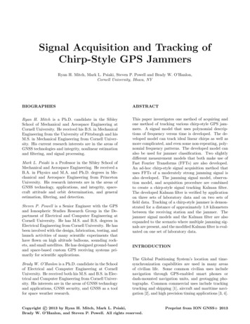
parameterization of a chirp-style jammer: θ f u α d α x A u t d t T(1)where the entries of the state vector are as follows: θ isthe phase in units of cycles, f is the frequency in unitsof Hertz, αu is the upward frequency rate of changein units of Hertz per second, αd is the downward frequency rate of change in units of Hertz per second, A isthe amplitude in units of Volts, tu is the ramp up timestart for the current ramp and is in units of seconds,td is the ramp down time start for the current rampand is in units of seconds, T is the chirp period and isin units of seconds. The ramp times could have separate periods, such as T u and T d , but experimentationwith separate periods did not dramatically change theresults presented later in this paper.Figure 2 A common GPS jammer spectrum. The topplot displays vertical slices of 64-point Hamming-windowed FFTs, and the bottom plot is of power.mation can be found in the survey of civilian GPSjammers in Ref. [8].JAMMER MODELING AND PARAMETERIZATIONThe above parameterization assumes that the jammerchirp has a linear first-order polynomial rate of changeof frequency versus time. For the majority of the chirpstyle jammers the above parameterization is a sufficiently accurate model for most signal processing algorithms. However, there are several jammers that havesignificantly different behavior. The following two figures show the spectra of two jammers that are notideally approximated by linear chirps. Fig. 4 appearsto have a non-first-order polynomial ramp down in frequency, whereas Fig. 5 has a non-first-order ramp upin frequency.There are multiple parameterizations that could be developed for the chirp-style jammer signal introduced inthe previous section. This paper considers a parameterization that is similar to that used in Ref. [15],but with several modifications. The parameterizationstarts by assuming a linear chirp, or a first-order rateof change of the frequency versus time, as shown inFig. 3.Figure 3 Time-history of the signal frequency of a linear first-order chirp, with appropriate states labeled.Figure 4 A jammer power spectra, with a non–first-order polynomial ramp down in frequency versustime.The following state vector is a moderately low-orderThe model state can be modified in several ways toaccount for higher-order variations in the frequency3
The general form of the new state vector is as follows: θ fu c1 . . u cMdu c1 (2)x . . cdMd A u t d tTFigure 5 A jammer power spectra, with a non–first-order polynomial ramp up in frequency versustime.All of the cuj and cdj states are coefficients of the Taylorseries-type polynomial expansion of the frequency behavior, including the first order terms cu1 and cd1 thathave replaced αu and αd . The states of the form cujare the coefficients of a ramp-up frequency polynomial,and the states of the form cdj are the coefficients ofa ramp-down frequency polynomial. The frequencypolynomial is defined as follows: MuX j cuj (t tu ) , tu tdf j 1f (x, t) (3)Md X j f cdj t td , td tu ramps. The modification method selected in this paperis to add new states that allow the frequency ramps tofollow higher-order polynomials, as is shown in Fig. 6.The polynomial expansion is in some ways analogousto a Taylor series expansion of a nonlinear term.j 1and it can be integrated to determine the corresponding phase:θ (x, t) MuX u (j 1) ) u θ f (t t ) cuj (t t(j 1), t u tdj 1Md X d (t td )(j 1) d θ f t t cj (j 1) , (4)tu tdj 1where the top case in Eqs. 3 and 4 is for times whenthe frequency is ramping upwards and the bottom caseis for times when the frequency is ramping downwards.The order of the polynomial, and the associated statescu1 –cuMu and cd1 –cdMd , can be considered a tuning parameter. More states will allow for a model that canmore closely replicate the behavior of the true jammer. The practical upper bound on the number ofcoefficients used in the model is primarily set by thesampling rate and numerical conditioning limitations.If the sampling rate is very low, then the number ofaccumulations that can be computed for each chirp isFigure 6 Possible time-history of the signal frequencyfor a polynomial-type chirp, with appropriate stateslabeled.4
reduced and it will be difficult to estimate the higherorder terms accurately. Numerical conditioning issuesmay arise due to the dramatically different state magnitudes in the above parameterization, and this mayrequire that the states be modified to improve the numerical stability of the algorithm. It should also benoted that using more polynomial coefficients thannecessary is a waste of computational effort. Therefore, the order of the polynomial should be limited toa reasonable number.process noise vector. The process noise is expected toenter only at the beginning of each ramp interval, tu ortd . It should be noted that the state transition matrixand the process noise influence matrix are both statedependent, and are defined as follows: if A Φ (tk 1 , tk )up ,(8)Φ (tk 1 , tk ; xk ) Φ (tk 1 , tk )down , if B I,otherwise if A Γ (tk 1 , tk )up ,(9)Γ (tk 1 , tk ; xk ) Γ (tk 1 , tk )down , if B otherwise0,A 5th order polynomial is considered for both the frequency ramp-up and ramp-down in the remainder ofthis paper’s modeling work. Additionally, the polynomial coefficients have been modified from the definition in Eqs. 2–4. The new polynomial coefficientshave been multiplied by the sample time Ts , raised tothe corresponding power, as shown below for the rampup:cu1,new .where the conditions A and B are defined as follows:(11)The state transition matrices for this system are theidentity matrices, except when Eqs. 10 and 11 are satisfied, i.e. when the system time equals td or tu . Whenthe system time equals td the phase and frequencyare propagated as defined by the up-ramp polynomialfrom time tu up to time td . Similarly, when the system time equals tu the phase and frequency are propagated as defined by the down-ramp polynomial fromtime td up to time tu . The time difference terms inEqs. 3 and 4 can be rewritten as rows of Φ (tk 1 , tk )upor Φ (tk 1 , tk )down because the states, the coefficientsof the polynomials, enter linearly into those equations.The amplitude, A, is defined as a constant and thetime states are defined by the following equations:(tu T, if t td(12)tu tu ,otherwise(td T, if t tutd (13)td ,otherwise(5)and for the ramp down:cd1,new cd1 (Ts )1.cdMd ,new cdMd (Ts )Md(10)uCondition B: t tcu1 (Ts )1cuMu ,new cuMu (Ts )MuCondition A: t td(6)The new states will have magnitudes that are closerto unity, and therefore will be less likely to cause numerical instabilities in the developed algorithms. Forexample, a reasonable numerical value for cu1 might be1012 , and a system with a sampling rate of 10 MHzwould cause cu1,new to have a numerical value closer to105 . It would also be possible to use a fixed numberthat is unrelated to sample rate.where the time states tu and td are incremented bytheir period T when the system time equals td or tu ,respectively. The rows corresponding to tu or td inΦ (tk 1 , tk )up or Φ (tk 1 , tk )down will have 1 entries forthat state, and if the conditions of Eqs. 10 or 11 aresatisfied, it will also have a 1 entry for the period increment for the corresponding state.The state dynamics are defined in a chirp-by-chirpmanner, with the frequency and phase defined at theramp times tu and td . The phase and frequency canbe evaluated at any time, but are only propagated forward and updated when the time crosses the rampdown time, td , or ramp-up time, tu , by evaluatingEqs. 3 and 4.Propagation of the state from a time before tu or tdto a time after tu or td will require multiple matrices.For example, if the state were propagated from time tkto tu and then from tu to tk 1 the resulting equationswould be: Φ (tk 1 , tk , xk ) Φ tk 1 , tu Φ tu , tu Φ tu , tkThe resulting state dynamics equation is as follows:xk 1 Φk (tk 1 , tk ; xk ) xk Γk (tk 1 , tk ; xk ) v k (7)where xk 1 is the state at time tk 1 , xk is the state attime tk , Φk is the state transition matrix from time tkto tk 1 , Γk is the process noise influence matrix, andv k is the zero-mean, unity-covariance, white, Gaussian I Φ (tk 1 , tk )down I Φ (tk 1 , tk )down5(14)
where the time tu designates a time infinitesimally before tu and time tu designates a time infinitesimally after tu . If multiple ramp changes were included in thepropagation interval then matrix multiplication seriesof Eq. 14 would contain more terms.JAMMER CLASSIFICATIONIn Ref. [8] the authors found that jammers with thesame physical appearances produced significantly different frequency versus time behavior. The unique frequency versus time behavior can potentially be usedto identify individual jammers. Jammer identificationcan be useful for determining how many different jammers are seen at one station. It can also be useful ifa person is being prosecuted for operating a PPD andthe authorities wish to know where else that personhas broken the law by jamming GPS. Jammer identification only requires that at least one station receivethe jamming signal, as opposed to most automatedgeolocation methods which require several stations.The default process noise influence matrices for thissystem are zero matrices, except when the conditionsin Eqs. 10 or 11 are met, i.e. when the system timeequals td or tu . All of the states, except for θ, areconsidered to have some process noise enter at the beginning of each ramp. The introduction of processnoise creates non-zero entries in the Γ matrices, whichare assumed to be diagonal. If the non-zero diagonalentries are each set to 1, then the process noise covariance matrix Q becomes the square of the standarddeviation of the process noise expected for the entireramp. Q is formally defined as: Q E[(v k E[v k ]) (v k E[v k ]) ] E[v k v k ]One possible identification method would be to storea short amount of time of high-sample-rate data frommany jammers in an RF signature library and thencompute cross correlations between the received dataand the library to determine if the signals match. Anew method using the modeling in this paper wouldalso start with a short recording of data from each jammer in the library. The jammer state would then beestimated for many chirps. The resulting time-seriesof state estimates would then comprise many samplesfrom a probability density function (pdf) of the jammer’s state perturbed by process noise. A similar procedure would then be applied to the new received signal and the resulting two sets of pdfs would be compared to each other. Relevant similarity metrics andhypothesis tests could be developed to determine ifthe new signal is the same as one of the signals in thelibrary. This method of jammer identification mightrequire a smaller amount of storage space when compared to one which used a sampled RF data library.This is a potentially deep research area and will requirefurther investigation to explore.(15)where E [] is the expected value of the quantity in thebrackets. A reasonable assumption for the Q matrixis that all of the noise inputs are uncoupled, i.e. Q isa diagonal matrix.The amount of process noise that is assumed to bepresent in each signal state is a tuning parameter thatcan be modified to improve the performance of the filter. The signal tracking results of the single GPS jammers were not extremely sensitive to the assumed levelof process noise. However, the multi-jammer scenarioswere decidedly more sensitive to the process noise tuning. It should be noted that each jammer can have adifferent level of process noise, and a thorough surveycould be conducted to determine a statistically significant estimate of the process noises that could beexpected from any GPS jammer seen in the field. Asurvey of that many jammers is beyond the scope ofthis current work.The resulting output of the above jammer model is:yi0 A0i cos(2π φ(x, ti ))JAMMER OBSERVABLES(16)where φ(x, ti ) is the evaluation of the relevant phasepolynomial, and A0i is the broadcast signal amplitude,at time ti . The signal as seen at a receiver station withmixing frequency fmix , and with the high-frequencymixing term removed, is as follows:Ai cos (2π (φ (x, ti ) fmix ti ))yi 2Ai cos (Θ (x, ti , fmix ))2The standard pair of observables used to track anRF signal are the In-Phase and Quadrature accumulations. The accumulation formulas at time tk are:Ik NX yi cos ΘN CO (ti )(18)yi sin ΘN CO (ti )(19)i 1(17)Qk NX i 1where the amplitude in Eq. 17 is the actual trackedamplitude state. Eq. 17 is the final form of the signalmodel that is used in the remainder of this paper.where N is the number of samples used in the accumulation, yi is the sampled RF data, and ΘN CO (ti ) is6
the numerically controlled oscillator (NCO) phase attime ti .time-histories are close to that of the real signal beingtracked.The NCO phase is arbitrarily defined by the user. Thejammer phase time history can be determined from theprevious modeling section and is as follows for a singlepolynomial ramp:The slow evaluation speed and a strong preference formultiple accumulations suggest that a different measurement model that does not have the same drawbacks should be considered. It should be noted that,unlike GPS, the GPS jammers broadcast very powerful signals, and their signal can be easily seen abovethe noise floor in a given area around each jammer. Afaster measurement that computes accumulations andspans the frequency range of the physical sampling system is the Fast Fourier Transform (FFT). The FFTcomputes accumulations at fixed frequencies spacedevenly between the positive and negative Nyquist frequency bounds. If the accumulation lengths are shortenough that they do not lose power due to the changing frequency of the incoming signal then they willprovide a measurement of the jammer power in eachfrequency bin across the entire Nyquist range.Θ (x, ti , fmix ) "2π θkN NAX fkN tA cAjj 1 # tj 1A fmix ti(j 1) (Ts )j(20)where the subscript “A” denotes ramp A, tA is defined as ti tA , and tA is either tu or td , depending onif the ramp is up or down, respectively. If the accumulation time interval spans part of two ramps, rampA and then ramp B, the phase is as follows:Θ (x, ti , fmix ) "2π θkN fkN tA NBXj 1cBj !j 1 t tBABAcA tBj(T)j (j 1)sj 1!#The FFT measurements are defined as follows:NAX tj 1B(j 1) (Ts )j fmix tiz(L) I iQ (21)NXw(n)y(n)e i2π(L 1)(n 1)Nn 1where tBA is defined as tB tA , and tB is either tuor td and tA is the other, i.e. if the first ramp is an upramp then ramp A starts at time tu and tB td . Ifmore than two ramps are spanned by an accumulationinterval then the received phase equation simply gainsadditional terms. NXw(n)y(n)e iζ(L,n,N )(22)n 1 L [1, ., N ]where w is the time domain windowing function usedto reduce sidelobes in the FFT, y is the sampled signal,and L is the frequency bin number of the FFT. Thepresent work used the Hamming window, but otherwindowing functions would likely produce similar results.If the signal contains no noise, then the NCO phasethat produces the largest accumulation is the samephase as the incoming signal that one wishes to track.In a traditional signal tracking architecture the accumulations would then constitute the measurementsthat would be sent to the Kalman filter. The corresponding measurement models would then be definedby substituting the signal model and the signal modelestimates into the yi term in the accumulation modelsof Eqs. 18 and 19. The measurement models can besimplified further by converting the discrete sums tocontinuous integrals and attempting to solve the resulting integrals in closed form. The integral of thehigher order phase terms is at simplest, in the case ofa perfectly linear ramp, a Fresnel integral. The higherorder polynomials will further complicate the integration. The resulting measurement model is complicatedand requires significant computational overhead. Additionally, a single pair of long time-span accumulations is likely to prove insufficient for filter convergenceand signal tracking. This is because the accumulationswill result in appreciable power only if the NCO phaseIt is important to note that it would be unreasonableto expect that the phase can be precisely tracked inthis system. Precise tracking of the phase state θ requires at least the following two conditions be met.The first condition is that the frequency polynomialestimate be very accurate, such that there are onlyvery minor fluctuations in the frequency that cannotbe modeled by the polynomial. The second conditionis that the jamming signal always stays within the receiver’s Nyquist frequency bounds.Satisfying the above two conditions will be difficult ineven the most benign situations, where the jammingenvironment can be controlled and RF data can beacquired with a high-speed recording system. The results of two such scenario are shown in Figs. 7 and 8.In Fig. 7 the order of the frequency polynomial required to describe the signal changes from chirp to7
chirp, and sometimes the frequency of the signal performs near-instantaneous jumps that may not be accurately modeled by a continuous polynomial. Evena well-designed signal tracking algorithm will therefore be unable to accurately track this jammer’s phase,unless the instantaneous jump behavior is accuratelymodeled and reliably estimated. The frequency polynomial model developed in this paper does not permitinstantaneous frequency jumps, but it will allow an approximation to that behavior. In Fig. 8 the frequencyof the jamming signal passes outside of the receiversystem’s Nyquist range. When the frequency passesoutside of the Nyquist range the phase can no longerbe tracked. Although the frequency and phase behavior are governed by the polynomial parameterizationsdeveloped in this paper, they are not guarantees of thebehavior outside of the visible frequency range. TheNyquist frequency range is dependent on the equipment being used, but even in the above high-rate laboratory system the signal is not always visible, and fieldequipment typically uses a lower digitization rate.Figure 8 A jammer power spectra, the frequencyspan is much greater than that covered by the high-speed data sampling equipment (62.5 MHz complexsamples). Phase estimates derived from data thatspans multiple ramps will likely be erroneous.The measurement model is defined similarly:h(L) I(x) (iQ(x)) NXw(n)ȳ(n, x, fmix )e iζ(L,n,N ) (24)n 1 L [1, ., N ]where ȳ is the predicted RF sample obtained by propagating the state to the current measurement intervaland evaluating Eq. 17 for the time at sample n. The Iand Q dependencies on the non-state terms have beenomitted for the sake of notational convenience. TheJacobian, or partial derivatives of the measurementmodel with respect to the model state, is required forKalman filter estimation and is defined as:Figure 7 A jammer power spectra, with jumps in frequency. Continuous approximations to the above frequency behavior will likely be inaccurate and the phaseestimate will likely be untrustworthy. I(x) (iQ(x)) xN X w(n)ȳ(n, x, fmix )e iζ(L,n,N ) x n 1H(L) Because the phase estimated state θ is unlikely to beaccurate, the phase state will be removed for the singlejammer signal tracking case. The resulting measurements are further simplified by considering only theabsolute value of the accumulations, as follows: L [1, ., N ]The absolute value is defined as: a (ib) z(L) I (iQ) NXw(n)y(n)e(25)p(a2 ) (b2 )(26)and the partial derivative as: iζ(L,n,N ) (23)n 1 a (ib) x L [1, ., N ]8a a x b a (ib) b x (27)
In the case of the measurement model from Eq. 24:The measurement model is defined as follows:a I (x) h(L) I(x)2 Q(x)2NX L [1, ., N ]Aw(n)cos (Θ(x, tn , fmix ) ζ (L, n, N ))2 n 1with partial derivatives:NAX w(n)cos (µ (L, n, N, fmix , x))2 n 1 NAXw(n)cos (µ (P , x))2 n 1 I(x)2 Q(x)2 x I(x) Q(x) 2I(x) 2Q(x) x x L [1, ., N ]H(L) (28)b Q (x)Every RF sample includes some amount of samplenoise, which eventually becomes accumulation noise.The noise statistics of the absolute value of the FFTsis complicated and only an approximation has beenused in this paper. The results are similar to the noisestatistics for the power measurements, which are asfollows: 2E[z(L)] Itrue Q2true N σ 2(35)NAX w(n)sin (µ (L, n, N, fmix , x))2 n 1NAXw(n)sin (µ (P , x))2 n 1(29)where P is a vector of parameters that has been introduced for notational convenience and includes L, n,N , andfmix . The reason that Eq. 28 and 29 are onlyapproximations is because the high frequency term,from the conversion of the products of the trigonometric terms to the sum of the terms with combinedarguments, is assumed to sum to zero. The resultingpartial derivatives of a and b are as follows: a, for x A A N aX (30)A x w(n) Θ x sin (µ (P , x)) , otherwise 2 cov(z(L)) E (z(L) E[z(L)]) (z(L) E[z(L)]) 2 2N σ 2 Itrue Q2true N 2 σ 4(36)where Itrue and Qtrue are the accumulations if thesignal contained zero noise.One component of the measurement model that stillneeds to be addressed is the RF filter characteristics ofthe physical jammers and recording devices. The RFfilters will attenuate different frequencies at differentrates. The data recording equipment RF filter shapecan be determined off-line. Off-line system identification is likely not possible for the jammers, becausethe equipment is not typically available before the firstencounter in the field. It might still be possible to perform off-line system identification on several jammersand attempt to identify repeatable RF filter shapesamong the surveyed jammers. Therefore, if the classof the jammer is known a priori then the RF filtershape can be assumed—it may provide sufficient accuracy for tra
eld data. Tracking of a chirp-style jammer is demon-strated for a distance of approximately 1.8 kilometers between the receiving station and the jammer. The jammer signal models and the Kalman lter are also expanded to the scenario where multiple jamming sig-nals are present, and the modi ed Kalman lter is eval-uated on one set of laboratory data.