Transcription
CalculusThis is the free digital calculus text by David R. Guichard and others. It wassubmitted to the Free Digital Textbook Initiative in California and will remainunchanged for at least two years.The book is in use at Whitman College and is occasionally updated to correcterrors and add new material. The latest versions may be found by going tohttp://www.whitman.edu/mathematics/california calculus/
This work is licensed under the Creative Commons Attribution-NonCommercial-ShareAlike License. Toview a copy of this license, visit http://creativecommons.org/licenses/by-nc-sa/3.0/ or send a letter toCreative Commons, 543 Howard Street, 5th Floor, San Francisco, California, 94105, USA. If you distributethis work or a derivative, include the history of the document.This text was initially written by David Guichard. The single variable material (not including infiniteseries) was originally a modification and expansion of notes written by Neal Koblitz at the Universityof Washington, who generously gave permission to use, modify, and distribute his work. New materialhas been added, and old material has been modified, so some portions now bear little resemblance to theoriginal.The book includes some exercises from Elementary Calculus: An Approach Using Infinitesimals, byH. Jerome Keisler, available at http://www.math.wisc.edu/ keisler/calc.html under a Creative Commons license. Albert Schueller, Barry Balof, and Mike Wills have contributed additional material.This copy of the text was produced at 16:02 on 5/31/2009.I will be glad to receive corrections and suggestions for improvement at guichard@whitman.edu.
Contents1Analytic Geometry1.11.21.31.41Lines . . . . . . . . . . . . . . . .Distance Between Two Points; CirclesFunctions . . . . . . . . . . . . . .Shifts and Dilations . . . . . . . . .2.7.8142Instantaneous Rate Of Change: The Derivative2.12.22.32.42.5The slope of a function .An example . . . . . . .Limits . . . . . . . . .The Derivative FunctionAdjectives For Functions.19.1924263540v
viContents3Rules For Finding Derivatives3.13.23.33.43.5The Power Rule . . . . .Linearity of the DerivativeThe Product Rule . . . .The Quotient Rule . . . .The Chain Rule . . . . . .45.45485053564Transcendental etric Functions . . . . . . . . . . . . . . . .The Derivative of sin x . . . . . . . . . . . . . . . . .A hard limit . . . . . . . . . . . . . . . . . . . . . .The Derivative of sin x, continued . . . . . . . . . . . .Derivatives of the Trigonometric Functions . . . . . . .Exponential and Logarithmic functions . . . . . . . . .Derivatives of the exponential and logarithmic functionsLimits revisited . . . . . . . . . . . . . . . . . . . . .Implicit Differentiation . . . . . . . . . . . . . . . . .Inverse Trigonometric Functions . . . . . . . . . . . .636667707172758084895Curve Sketching5.15.25.35.45.5Maxima and Minima . . . . . . . . . . .The first derivative test . . . . . . . . . .The second derivative test . . . . . . . .Concavity and inflection points . . . . . .Asymptotes and Other Things to Look For93. . 93. . 97. . 99. 100. 102
Contentsvii6Applications of the Derivative6.16.26.36.46.5Optimization . . . . . . .Related Rates . . . . . .Newton’s Method . . . . .Linear Approximations . .The Mean Value Two examples . . . . . . . . . . . . . . . . . . . . . . . . .The Fundamental Theorem of Calculus . . . . . . . . . . . . .Some Properties of Integrals . . . . . . . . . . . . . . . . . .1391431508Techniques of Integration8.18.28.38.48.58.6Substitution . . . . . . .Powers of sine and cosine .Trigonometric SubstitutionsIntegration by Parts . . .Rational Functions . . . .Additional exercises . . . .155.156160162166170176
viiiContents9Applications of rea between curves . . . . . . .Distance, Velocity, Acceleration . .Volume . . . . . . . . . . . . . .Average value of a function . . . .Work . . . . . . . . . . . . . . .Center of Mass . . . . . . . . . .Kinetic energy; improper integralsProbability . . . . . . . . . . . .Arc Length . . . . . . . . . . . .Surface Area . . . . . . . . . . .Differential equations . . . . . . .17718218519219520020521022022222710Sequences and 1110.12Sequences . . . . . . . . .Series . . . . . . . . . . .The Integral Test . . . . .Alternating Series . . . . .Comparison Tests . . . . .Absolute Convergence . .The Ratio and Root TestsPower Series . . . . . . .Calculus with Power SeriesTaylor Series . . . . . . .Taylor’s Theorem . . . . .Additional exercises . . . .233.234240244249251254256259261263267271
ContentsixAIntroduction to MapleA.1A.2Getting Started . . . . . . . . .Algebra . . . . . . . . . . . . .A.2.1 Numbers . . . . . . . . . .A.2.2 Variables and Expressions . .A.2.3 Evaluation and SubstitutionA.2.4 Solving Equations . . . . .A.3Plotting . . . . . . . . . . . .A.4Calculus . . . . . . . . . . . .A.4.1 Limits . . . . . . . . . . .A.4.2 Differentiation . . . . . . .A.4.3 Implicit Differentiation . . .A.4.4 Integration . . . . . . . . .A.5Adding text to a Maple session .A.6Printing . . . . . . . . . . . .A.7Saving your work . . . . . . . .A.8Getting Help . . . . . . . . . .275. . . 276. 277. 279. 280. . . 284. 284. 285. 285. . . . .275276282284286286286287BSelected Answers289Index303
IntroductionThe emphasis in this course is on problems—doing calculations and story problems. Tomaster problem solving one needs a tremendous amount of practice doing problems. Themore problems you do the better you will be at doing them, as patterns will start to emergein both the problems and in successful approaches to them. You will learn fastest and bestif you devote some time to doing problems every day.Typically the most difficult problems are story problems, since they require some effortbefore you can begin calculating. Here are some pointers for doing story problems:1. Carefully read each problem twice before writing anything.2. Assign letters to quantities that are described only in words; draw a diagram ifappropriate.3. Decide which letters are constants and which are variables. A letter stands for aconstant if its value remains the same throughout the problem.4. Using mathematical notation, write down what you know and then write downwhat you want to find.5. Decide what category of problem it is (this might be obvious if the problem comesat the end of a particular chapter, but will not necessarily be so obvious if it comeson an exam covering several chapters).6. Double check each step as you go along; don’t wait until the end to check yourwork.xi
xiiIntroduction7. Use common sense; if an answer is out of the range of practical possibilities, thencheck your work to see where you went wrong.Suggestions for Using This Text1. Read the example problems carefully, filling in any steps that are left out (asksomeone if you can’t follow the solution to a worked example).2. Later use the worked examples to study by covering the solutions, and seeing ifyou can solve the problems on your own.3. Most exercises have answers in Appendix B; the availability of an answer is markedby “ ” at the end of the exercise. In the pdf version of the full text, clickingon the arrow will take you to the answer. The answers should be used only asa final check on your work, not as a crutch. Keep in mind that sometimes ananswer could be expressed in various ways that are algebraically equivalent, sodon’t assume that your answer is wrong just because it doesn’t have exactly thesame form as the answer in the back.4. A few figures in the book are marked with “(JA)” at the end of the caption.Clicking on this should open a related Java applet in your web browser.Some Useful FormulasAlgebraRemember that the common algebraic operations have precedences relative to eachother: for example, mulitplication and division take precedence over addition andsubtraction, but are “tied” with each other. In the case of ties, work left to right. Thismeans, for example, that 1/2x means (1/2)x: do the division, then the multiplicationin left to right order. It sometimes is a good idea to use more parentheses than strictlynecessary, for clarity, but it is also a bad idea to use too many parentheses.Completing the square: x2 bx c (x 2b )2 b24 c. b b2 4acQuadratic formula: the roots of ax2 bx c are.2aExponent rules:ab · ac ab cab ab ccab c(a ) abc a1/b b a
IntroductionxiiiGeometryCircle: circumference 2πr, area πr2 .Sphere: vol 4πr3 /3, surface area 4πr2 .Cylinder: vol πr2 h, lateral area 2πrh, total surface area 2πrh 2πr2 . Cone: vol πr2 h/3, lateral area πr r2 h2 , total surface area πr r2 h2 πr2 .Analytic geometryPoint-slope formula for straight line through the point (x0 , y0 ) with slope m: y y0 m(x x0 ).Circle with radius r centered at (h, k): (x h)2 (y k)2 r2 .x2y2Ellipse with axes on the x-axis and y-axis: 2 2 1.abTrigonometrysin(θ) opposite/hypotenusecos(θ) adjacent/hypotenusetan(θ) opposite/adjacentsec(θ) 1/ cos(θ)csc(θ) 1/ sin(θ)cot(θ) 1/ tan(θ)tan(θ) sin(θ)/ cos(θ)cot(θ) cos(θ)/ sin(θ) ¡sin(θ) cos π2 θ¡ cos(θ) sin π2 θsin(θ π) sin(θ)cos(θ π) cos(θ)Law of cosines: a2 b2 c2 2bc cos ALaw of sines:bca sin Asin Bsin C
xivIntroductionSine of sum of angles: sin(x y) sin x cos y cos x sin ysin2 (θ) and cos2 (θ) formulas:sin2 (θ) cos2 (θ) 11 cos(2θ)21 cos(2θ)cos2 (θ) 2sin2 (θ) Cosine of sum of angles: cos(x y) cos x cos y sin x sin yTangent of sum of angles: tan(x y) tan x tan y1 tan x tan y
1Analytic GeometryMuch of the mathematics in this chapter will be review for you. However, the exampleswill be oriented toward applications and so will take some thought.In the (x, y) coordinate system we normally write the x-axis horizontally, with positivenumbers to the right of the origin, and the y-axis vertically, with positive numbers abovethe origin. That is, unless stated otherwise, we take “rightward” to be the positive xdirection and “upward” to be the positive y-direction. In a purely mathematical situation,we normally choose the same scale for the x- and y-axes. For example, the line joining theorigin to the point (a, a) makes an angle of 45 with the x-axis (and also with the y-axis).But in applications, often letters other than x and y are used, and often different scalesare chosen in the x and y directions. For example, suppose you drop something from awindow, and you want to study how its height above the ground changes from second tosecond. It is natural to let the letter t denote the time (the number of seconds since theobject was released) and to let the letter h denote the height. For each t (say, at one-secondintervals) you have a corresponding height h. This information can be tabulated, and thenplotted on the (t, h) coordinate plane, as shown in figure 1.1.We use the word “quadrant” for each of the four regions the plane is divided into: thefirst quadrant is where points have both coordinates positive, or the “northeast” portionof the plot, and the second, third, and fourth quadrants are counted off counterclockwise,so the second quadrant is the northwest, the third is the southwest, and the fourth is thesoutheast.1
2Chapter 1 Analytic Geometryseconds01234meters8075.160.435.91.6h80 604020. 01Figure 1.123t4A data plot.Suppose we have two points A(2, 1) and B(3, 3) in the (x, y)-plane. We often wantto know the change in x-coordinate (also called the “horizontal distance”) in going fromA to B. This is often written x, where the meaning of (a capital delta in the Greekalphabet) is “change in”. (Thus, x can be read as “change in x” although it usuallyis read as “delta x”. The point is that x denotes a single number, and should not beinterpreted as “delta times x”.) In our example, x 3 2 1. Similarly, the “change iny” is written y. In our example, y 3 1 2, the difference between the y-coordinatesof the two points. It is the vertical distance you have to move in going from A to B. Thegeneral formulas for the change in x and the change in y between a point (x1 , y1 ) and apoint (x2 , y2 ) is: x x2 x1 , y y2 y1 .Note that either or both of these might be negative.1.1 LinesIf we have two points A(x1 , y1 ) and B(x2 , y2 ), then we can draw one and only one linethrough both points. By the slope of this line we mean the ratio o
” at the end of the exercise. In the pdf version of the full text, clicking on the arrow will take you to the answer. The answers should be used only as a final check on your work, not as a crutch. Keep in mind that sometimes an answer could be expressed in various ways that are algebraically equivalent, so