Transcription
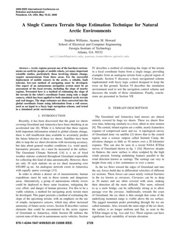
2008 IEEE International Conference onRobotics and AutomationPasadena, CA, USA, May 19-23, 2008A Single Camera Terrain Slope Estimation Technique for NaturalArctic EnvironmentsStephen Williams, Ayanna M. HowardSchool of Electrical and Computer EngineeringGeorgia Institute of TechnologyAtlanta, GA 30332swilliams8@gatech.edu, ayanna.howard@ece.gatech.eduAbstract— Arctic regions present one of the harshest environments on earth for people or mobile robots, yet many importantscientific studies, particularly those involving climate change,require measurements from these areas. For the successfuldeployment of mobile sensors in the arctic, a reliable, faulttolerant, low-cost method of navigating must be developed.One aspect of an autonomous navigation system must be anassessment of the local terrain, including the slope of nearbyregions. Presented here is a method of estimating the slope ofthe terrain in the robot’s coordinate frame using only a singlecamera, which has been applied to both simulated arctic terrainand real images. The slope estimates are then converted into theglobal coordinate frame using information from a roll sensor,used as an input to a fuzzy logic navigation scheme, and testedin a simulated arctic environment.IV describes a method of estimating the slope of the terrainin a local coordinate frame from a single image, providingexamples from an analogous terrain from a glacial region ofColorado. Section V discusses a basic navigational schemeimplemented with fuzzy logic control designed to keep therover on flat ground. Section VI describes the simulationenvironment used to test the navigation control scheme anddiscusses the results of those simulations. Finally, conclusions are presented in Section VII.I. INTRODUCTIONThe Greenland and Antarctica land masses are almostentirely covered by huge ice sheets. These ice sheets flowover time, behaving similarly to a river, albeit in slow motion[8]. The central, inland regions are a stable, nearly featurelessexpanse of compressed snow and ice. A topological surveyof Greenland done via satellite [3] shows that in the centralregion, near a science outpost called Summit Camp, theelevation changes as little as 10 meters over a 20 kilometerexpanse. This can also be seen in a recent NASA ICESatsurvey of Greenland shown in fig. 1 [16]. However, despiteits flatness, the snow surface is often sculpted by the highwinds present, forming undulating features parallel to thewind direction known as sastrugi. The sastrugi can vary inheight from only a few centimeters to over a meter.As the ice flows toward the edges of Greenland and intothe sea, forces build due to differential velocities of differentice sections. These forces can cause nearly vertical fracturesin the ice known as crevasses. Crevasses can be as deepas 30 meters and are often covered with snow, makingtheir detection all the more difficult. This snow, referredto as a snow bridge, can be sufficiently strong as to allowpassage over the crevasse. Additionally, towards the coastof Greenland, the ice sheet is thin enough that some of theunderlying mountain range is visible above the ice surface.The jagged mountain peaks protruding through the ice arecalled nunataks. Also, towards the outer edge of the ice sheet,the surface is no longer uniform and flat, as seen in theICESat images in fig. 1(a) and 1(c). These regions can havesignificant local variability of terrain elevation.Recently, it has been discovered that the giant ice sheetscovering Greenland and Antarctica have been shrinking at anaccelerated rate [6]. While it is believed that these regionshold important information related to global climate change,there is still insufficient data available to accurately predictthe future behavior of these ice sheets. Satellites have beenable to map the ice sheet elevations with increasing accuracy,but data about general weather conditions (i.e. wind speed,barometric pressure, etc.) must be measured at the surface.The Greenland Climate Network [14] is a set of fixedweather stations scattered throughout Greenland responsiblefor collecting this kind of data automatically. However, thereare only 18 such stations on an ice sheet measuring over650,000 sq mi. An analogous network exists in Antarcticawith equally sparse coverage [13].In order to obtain a denser set of measurements, humanexpeditions must be sent to these remote and dangerousareas. Alternatively, a group of autonomous robotic roverscould be deployed to these same locations, mitigating thecost, effort, and danger of human presence. For this to be aviable solution, a method for navigating arctic terrain mustbe developed. This paper presents a method of estimating theslope of the upcoming terrain, with an emphasis on the useof simple, inexpensive sensors, which may allow increasedautonomy of future arctic rovers. Section II describes variouselements that could be encountered in the arctic regionsof Greenland or Antarctica, while Section III outlines thecurrent state-of-the-art in autonomous arctic vehicles. Section978-1-4244-1647-9/08/ 25.00 2008 IEEE.II. TERRAIN DESCRIPTION2729
(a)(b)(c)Fig. 1. (a) A high resolution elevation map of Greenland from ICESat [16], (b) an enlarged view of the nearly featureless area in the center of the icesheet near Summit Camp, and (c) an enlarged view of a north-western section of the ice sheet near Qaanaaq illustrating an area of more rugged terrain.III. BACKGROUND ON ARCTIC RESEARCHWhile the arctic possesses significant information of scientific value, surprisingly little research is devoted to creating mobile, autonomous robots to collect this data. TheCoolRobot [12] developed by Dartmouth College is designedto be a mobile sensor station for use on the Antarcticplateau. This region is essentially featureless, lacking anyknown obstacles or elevation changes that could impede therobot’s motion. Consequently, the navigation system consistssolely of a GPS unit and a simple waypoint followingalgorithm. It has been successfully tested at an analogoussite in Greenland, where it operated autonomously for up toeight hours [9].The Nomad project [2] at Carnegie Melon University wasdesigned for autonomous meteorite location in the Antarcticmoraines. The Elephant Moraine, where the Nomad wasdeployed, is essentially a sheet of blue ice littered withrocks ranging in size from pebbles to large boulders. Dueto the search and classify nature of the Nomad’s mission, itnaturally requires greater sensing capability, and has beenoutfitted with a high resolution steerable camera, stereocameras, a scanning laser range finder, and a pitch-roll-yawsensor, as well as a scientific instrumentation package. Thus,the navigational system of the Nomad is more complex thanthat of the CoolRobot, consisting of a GPS waypoint system,an obstacle avoidance system based on the laser rangefinder data, a potential meteorite targeting system basedon camera images, and a management system to gracefullyswitch between the different modes. However, due to theknown flatness of the testing and deployment environment,little in way of terrain assessment is required for successfulnavigation. It has been deployed several times to Antarctica,during which it has autonomously found and identified 5meteorites.The University of Kansas is developing an autonomoussnowmobile-based rover for taking ice sheet measurementsas part of the PRISM project [5]. Like the Nomad, it isequipped with a camera system as well as a laser rangefinder for obstacle detection and avoidance. However, unlikethe Nomad or CoolRobot, the use of a snowmobile chassisallows for a much wider range of navigable terrain. However,during operation, the PRISM rover will follow, or performpredefined maneuvers, behind a manned unit. Consequently,obstacle avoidance is sufficient in this case, relying on thehuman operator to set the lead course through acceptableregions. Similarly, the ENEA R.A.S. project [4] has thegoal of creating an automated convoy of snowcats, largetracked vehicles, in which the lead vehicle is driven by ahuman. Again, the snowcats have the capability of traversingsignificant inclines and can be used in a wide range of arcticterrain, but the determination of acceptable terrain is leftsolely to the lead human driver.IV. SLOPE EXTRACTIONCurrently, most autonomous driving research is basedupon laser range finders or stereo cameras which returnquantitative depth information. In contrast, humans navigate through an enormous variety of cluttered environmentswithout explicitly using any such depth data. Instead, werely on qualitative information, such as “Those mountainsare far away”, or “That rock is close.” Visual cues in ourenvironment, such as relative height and position relativeto the horizon, are used to help determine the nature anddistance of objects in our field of view. A method ofestimating the terrain slope of an arctic scene is outlinedbelow. Similar to human perception, this method relies onvisual cues from a single camera to make its estimates. Allimage processing was done in C and utilized the OpenCVlibraries [1].A. Region ExtractionThe first step is to extract the region of the image to beanalyzed. Such things as distant mountains, clouds, trees,2730
(a)(b)(c)(d)(e)Fig. 2. (a) A sample arctic image from Colorado, (b) the histogram of the sample image with the adaptive thresholds indicated, and (c) the resultingbinary mask. (d) The results of a bandpass filter and Canny edge detector on the sample image, and (e) the final slope estimates superimposed on theoriginal image.and peripheral views of the rover itself can interfere withthe estimation process. A method of histogram thresholding,suggested in [4], has been adopted here. It is assumed thatthe majority of the image is filled with the snowy region.Consequently, in the histogram of the image, the largest peakshould be associated with the grayscale values of this region.Thus, an adaptive threshold based on the boundaries of thispeak can effectively separate the region of interest fromunwanted objects and areas. To locate the peak boundaries,the grayscale image histogram is first computed and themaximum value located. Then, the histogram is searched inboth directions for local minima. Criteria on the number ofpoints between consecutive local minima is used to makethe process more robust to noise. The two grayscale valuesfound are used to threshold the image, creating a binarymask. The mask is then eroded by several pixels to ensure theedges of the unwanted features are concealed by the mask.Fig. 2 shows a representative image from a glacial regionin Colorado, followed by its histogram with the thresholdlimits, and the resulting mask.B. Texture FilteringA human is able to quickly and accurately estimate theslope of the environment, such as that shown in fig. 2(a).From this single image, without any depth information, onecan successfully estimate slope and loosely define distancesfrom the camera (such as “close” or “far”). One of the keysin our ability to estimate the slope comes from visual cuesin the form of light and dark streaks in the snow that arealigned with the perceived slope. These features are of thegreatest interest in the slope estimation process.The dark and light striations are clearly visible and con-siderably larger in scale than the snow texture. However,these striations are far from uniform in the region of interest.Clearly then, these features exist in a mid-band of spatialfrequency, and can be effectively isolated using a simplebandpass filter. Filters based on Gaussian kernels are generally less likely to produce unwanted ringing effects. Additionally, since Gaussian kernels are linearly separable, thefilter can be applied in a computationally efficient manner.Experimentation with the Gaussian standard deviation, σ, ofthe low pass and high pass filter components has shown thata wide range of values have acceptable performance, but thevalues are dependent on the image size. Using a σ valuefor the high pass filter of twice that of the low pass filtergenerally produces good results. One final step in preparingthe image for slope estimation is to convert it into a binaryimage. This is done by applying a Canny edge detector tothe filtered image. The image after these processing stepscan be seen in fig. 2(d).C. Hough TransformIn the final step, the slope of the extracted features isestimated using a Hough transform, which transforms eachpixel in the image space into a sinusoidal line in the rhotheta parameter space. As each image pixel is transformed,the sinusoids in the parameter domain will tend to intersectif the image pixels are in a straight line. The number ofsinusoids that intersect in a particular location is an indicationof the strength or confidence of the line. Thus, the rho-thetapair corresponding to the maximum confidence values in theparameter space can be selected as being representative ofthat region. When the pixel is transformed into the parameterspace, it loses any sense of its location in the original2731
image. It is therefore common for many local maxima tooccur in a very small neighborhood. This results in havingslope data only for a small area in the total region ofinterest. To overcome this problem, the image is dividedinto smaller subimages, and the Hough transform is appliedseparately to each subimage. In this way, the extracted slopecan be applied to a specific area of the original image,and slope data will exist for all areas in the image. Ineach subarea, only one slope is desired, lending itself tothe Fast Hough Transform algorithm [10] which employsinteger shifts instead of floating point operations, reducingthe processing time considerably. The final image with thedetected slopes is shown in fig. 2(e).slope estimates generated in the grassy areas are generallyless stable than those of uninterrupted snow. In fig. 3(e) aset of snowmobile tracks is present which exhibit similarproperties to the surface striations, and are consequentlydetected by the slope estimate. A method to detect thepresence of tracks and mask them from the slope estimatewould be beneficial. Finally, fig. 3(f) shows an image with alower than normal amount of texture or prominent striations.This process is not able to produce estimates for the fullimage under these conditions, providing information onlywhere a certain level of confidence is met.V. NAVIGATION CONTROL SCHEMESince no measurement of the terrain is being taken, as isdone with a laser range finder or a stereo camera system,the output of this process is, at best, an estimate of theterrain. Thus, any navigation or control scheme based onthese estimates must be able to handle the inherent noise anduncertainty present in the results. Additionally, attempting tonavigate through natural terrain using only vision as an inputis something that humans have developed heuristically [7]. Acontrol scheme that could capture this inherently nonlinearheuristic knowledge would be advantageous. Fuzzy logiccontrol provides just such features [11], as well as modelsan input in terms of a linguistic set, such as “near” and“far”, which parallels how humans think in terms of theirenvironment.The first step is to convert the slope estimates into fuzzylinguistic sets. For the slope estimates, the following fivesets are used to classify each input: Positive Steep, PositiveSloped, Flat, Negative Sloped, and Negative Steep. Also,when the slope estimates were created, the original imagewas divided into an 8x8 grid, producing up to 64 slopevalues. In an attempt to reduce the number of inputs to aD. ResultsThe slope extraction process was then applied to a setof images taken in a glacial region in Colorado. Fig. 3(a)shows a snowmobile in the foreground of the image. Theestimation process ignored the area around the snowmobileand returned correct results for the surrounding regions,illustrating that the masking process can successfully removeunwanted objects from the analysis, particularly man-madeobjects. Fig, 3(d), however, illustrates the inability of thisprocess to remove unwanted regions, such as gray clouds,which exist in the same color range as the snow, thuscreating fictitious slope estimates. The estimation processdoes seem to be relatively immune to light intensities, asshown in fig. 3(b) and 3(c). These images show the samescene under different lighting conditions, with the secondshowing significantly more reflected light evidenced by theshiny appearance of the snow. Despite the different lightingconditions, the slope estimates seem stable and accurate. Themasking and estimation process are even partially successfulin the region of sparse grass shown in fig. 3(d). However, the(a)(b)(c)(d)(e)(f)Fig. 3.Slope estimates performed on a variety of images from a glacial region in Colorado.2732
manageable number, a 2x2 square of available slopes wereaveraged together reducing the total number to 16. Further,the uppermost row of data generally corresponds to the sky,clouds, or distant mountains. This row of data is ignoredby the control system, and, in practice, not calculated at all,bringing the final input count to 12.A fuzzy rule base was generated in terms of IF-THENstatements to control the robot’s direction. A human expertwas used to generate a set of simple rules with the intentionof keeping the robot driving on level ground. Due to symmetry, the rules that are used to turn right mirror the rulesto turn left. A total of seven rules, and their correspondingmirrors, were implemented as part of the fuzzy rule base.VI. SIMULATIONTo validate the fuzzy logic navigational control system, a simulated arctic terrain was produced using thePlayer/Stage/Gazebo project [15], an open source, physicsbased, 3-D simulation and control package. A series of elliptical hills were placed in the terrain, requiring the robot tomake many course corrections in both directions to maintaina level orientation. A topographical map of the simulatedterrain is shown in fig. 4(a). A synthetic texture file was thengenerated, mimicking the dark and light striations present inthe actual scenes, and wrapped around the terrain. Fig. 4(b)and 4(c) show the rover in the simulated environment andthe augmented view from the rover’s camera respectively.A. Navigational TrialsAs long as the rover remains on level ground, the camera’sreference frame and global frame will have the same orientation. However, if any body roll is introduced, the valuesdefined as F lat are offset from the global reference frame.As single chip multi-axis inclinometers are inexpensive andreadily available, measuring this value seems reasonable.A simulated roll-pitch-yaw sensor was added to the rover,allowing the slope estimates to be transformed back into theglobal reference frame.Multiple tests were conducted with the rover’s startingposition selected at various locations, summarized in TableI. The paths the rover traversed during select trials aresuperimposed on the elevation map in fig. 4(a). When therover is initialized on level ground, as was done in trials 1,2, 3, and 6, the resulting paths remain on level ground and(a)TABLE IE XPERIMENT D ESCRIPTIONExperiment123456Descriptionentrance to the course, starting on level groundentrance to the course, starting on level groundentrance to the course, starting on level groundmiddle of the course, starting on top of hillmiddle of the course, surrounded by hillsend of the course, starting on level groundeven converge after a short time, demonstrating the robustnature of the control laws. When the rover began on top of ahill, as shown in trial 4, the rover initially turned away fromthe edge, preferring the flatter section of hill’s apex. Oncethe rover entered the steep, downhill section, the rover turneddirectly into the slope, reducing the amount of body rollexperienced. Immediately after returning to the level area,the rover’s heading was sufficiently different from those ofthe other trials, which were required to navigate around thehill. This was sufficient to cause the path around the next hillto deviated from the standard path of trials 1-3. However,after this turn, the rover rejoins the standard route. Finally,when the rover was initialized in an area surrounded by hills,as was done in trial 5, the rover was able to successfullynavigate out and return to the standard route. During theU-turn maneuver required, the rover drives on the shallowoutskirts of one of the hills. Due to the minimal slope inthis region, the controller lacks sufficient incentive to correctthe path immediately. However, as the slope increases, thecontroller makes an additional path correction, returning itto the standard route.B. Numerical ResultsThe slope estimates of the real arctic images presentedin Section IV could only be evaluated qualitatively, as theground truth information could not be obtained. Within thesimulated environment, however, ground truth data was generated, which allowed for quantitative evaluation. Although,it should be noted that as this is a purely visual technique,the slope estimates are sensitive to the level of realismprovided by the simulation. Consequently, the followinganalysis should be viewed only as an indication of potentialperformance.(b)(c)Fig. 4. (a) A topological map of the simulated terrain with the rover paths superimposed, (b) an illustration of the rover situated in the simulatedenvironment, and (c) the rover’s view of the environment with slope estimates.2733
analysis area, but sections of unwanted natural objects, suchas clouds, often remain. Also, tracks left in the snow, whichis an inevitable condition for arctic rovers, are spuriouslyreported as part of the terrain slope. A method to locatesnow tracks and remove them from the processing regioncould greatly improve the effectiveness of the algorithm asa tool for field robotics.ACKNOWLEDGMENTSFig. 5.A plot of the visual slope estimates versus the ground truth data.The slope estimates generated by this method are twodimensional in nature. However, the actual landscape is athree dimensional entity which can exhibit different slopecharacteristics in each of those dimensions. When the rover’scamera views the landscape, the three dimensional terrain isprojected onto a two dimensional plane perpendicular to thecamera’s line of sight. In order to generate ground truth forthe simulation that would be comparable, a similar approachwas followed. For each slope estimate, a ray was projectedfrom the camera to a terrain patch at the center of the slopeestimate line. Once the intersection of this ray and the terrainis determined, the elevation of the terrain on either side ofthe intersection point is measured. The ground truth slope isthen calculated from the two measured elevations.With the data collection method in place, the rover wasdriven manually through a section of the simulated terrainwhile the generated visual slope estimates and ground truthdata were logged approximately once per second. Fig. 5shows a comparison between the ground truth data andthe visual slope estimates obtained during a 60 secondtraverse. As can be seen, the visual slope estimates are highlycorrelated with the ground truth data, with a correlationfactor above 0.9. The best fit line has a slope of 0.86,indicating that this method tends to mildly underestimate thelarger slopes. Over the data set presented, the error betweenthe estimate and ground truth value exhibits a near-zeromean, with a standard deviation of less than 3.0 degrees. Theestimates therefore provide a good indication of the terrainslope, which is supported by the success of the navigationtrials mentioned above.VII. CONCLUSIONSThe method outlined in this paper for terrain slope extraction has been shown to be effective both on imagesof real terrain, and as the input to a real-time fuzzy logicnavigational control scheme. The fuzzy logic frameworkprovides adequate performance even with the inherent estimation error, as well as provides a convenient methodfor translating heuristic human knowledge into control laws.The feature masking approach, originally presented in [4], isparticularly effective at removing man-made objects from theThis work was supported by the National Aeronautics andSpace Administration under the Earth Science and Technology Office, Applied Information Systems TechnologyProgram. The authors would also like to express their gratitude to our collaborators Dr. Derrick Lampkin, PennsylvaniaState University, for providing the scientific motivation forthis research and Dr. Magnus Egerstedt, Georgia Instituteof Technology, for providing his experience in multi-agentformations.R EFERENCES[1] D. Abrosimov et al. (2006, Feb) Opencv. intel open source computervision library. [Online]. Available: ndex.htm[2] D. Apostolopoulos, M. D. Wagner, B. Shamah, L. Pedersen, K. Shillcutt, and W. R. L. Whittaker, “Technology and field demonstrationof robotic search for antarctic meteorites,” International Journal ofRobotics Research, Dec 2000.[3] R. A. Bindschadler et al., “Surface topography of the greenland icesheet from satellite radar altimetry,” National Aeronautics and SpaceAdministration, Tech. Rep. NASA SP-503, 1989.[4] A. Broggi and A. Fascioli, “Artificial vision in extreme environmentsfor snowcat tracks detection,” IEEE Transactions on Intelligent Transportation Systems, vol. 3, pp. 162–172, Sep 2002.[5] S. Brumwell and A. Agah, “Mobility, autonomy, and sensing formobile radars in polar environments,” Information Telecommunicationand Technology Center, University of Kansas, Lawrence, KS, Tech.Rep. ITTC-FY2003-TR-20272-02, Nov 2002.[6] J. L. Chen, C. R. Wilson, and B. D. Tapley, “Satellite gravitymeasurements confirm accelerated melting of greenland ice sheet,”Science, Sept 2006.[7] A. Howard and H. Seraji, “Vision-based terrain characterization andtraversability assessment,” Journal of Robotic Systems, vol. 18, pp.577–587, Oct 2001.[8] P. G. Knight, Ed., Glacier Science and Environment Change. Blackwell Publishing, 2006.[9] J. Lever, A. Streeter, and L. Ray, “Performance of a solar-poweredrobot for polar instrument networks,” in Proceedings of the 2006IEEE International Conference on Robotics and Automation, Orlando,Florida, May 2006, pp. 4252–4257.[10] H. Li, M. A. Lavin, and R. J. L. Master, “Fast hough transform:A hierarchical approach,” Comput. Vision Graph. Image Process.,vol. 36, no. 2-3, pp. 139–161, 1986.[11] K. M. Passino and S. Yurkovich, Fuzzy Control. Addison-Wesley,1998.[12] L. Ray, A. Price, A. Streeter, D. Denton, and J. Lever, “The design ofa mobile robot for instrument network deployment in antarctica,” inProceedings of the 2005 IEEE International Conference on Roboticsand Automation, Barcelona, Spain, April 2005, pp. 2111–2116.[13] C. Stearns et al. (2004, March) Automatic weather stations projectand antarctic meteorological research center. [Online]. Available:http://amrc.ssec.wisc.edu/index.html[14] K. Steffen, J. E. Box, and W. Abdalati. (2005, Feb) Greenlandclimate network (gc-net). [Online]. Available: cnet/[15] R. T. Vaughan, B. Gerkey, and A. Howard. (2007, Aug)The player/stage project. [Online]. Available: http://playerstage.sourceforge.net/[16] H. J. Zwally and J. DiMarzio. (2005, June) Icesat home page.[Online]. Available: http://icesat.gsfc.nasa.gov/2734
Arctic Environments Stephen Williams, Ayanna M. Howard School of Electrical and Computer Engineering Georgia Institute of Technology Atlanta, GA 30332 swilliams8@gatech.edu, ayanna.howard@ece.gatech.edu Abstract Arctic regions present one of the harshest environ-ments on earth for people or mobile robots, yet many important