Transcription
Stat 200 Exam 2 Study Guide Updated covering Chapters 21-41The only 2 formulas that will be given to you on Exam 2 are:SDerrors 1 r2* SDyandSEslope SD errorsn *SD x2 1 r * SD yn * SD xFormulas not given to you that you need to know: Slope of the regression line rSD ySDn Z Zxy Correlation Coefficient, r Z and t test stats for testing H0 : slope 0 in simple regression (1 slope):Z r1 r 2i 1n* nt (n 2) r1 r 2* n 2NOTE: The Z and t formulas are the same as the square root of the χ2 and F formulas below when p 2. Chi square and F stats for testing H0 : All slopes 0 in multiple regressionχ2(p 1)R2 *n1 R 2R2n pF(p 1,n p) *21 R p 1 ANOVA for regression: SST SSM SSE and ANOVA for group means SST SSB SSW (seesummary on p.175) Formulas on page 186 for testing group means using:SE diff SD errors1 1and Bonferoni corrected p-values p-value * g(g-1)/2 n1 n 2For regression: #parameters (p) # of β’s in regression equation, for means: # parameters (p) # of groups (g)SourceSS (Sum ofSquares)ModelR 2SSTSSM (reg)SSB (means)Error(1 R 2 )SSTTotalSSE (reg)SSW (means)SSTdfp-1g-1n-pn-gn-11
Stat 200 Exam 2 Study Guide Updated covering Chapters 21-41Part VIII Simple Regression: Chapters 21-23Question 1 pertains to the 4 scatter plots below:Write the letter of the plot next to the correlation coefficient that is closest to it.a) r 0.36b) r 0.9c) r -0.79d) r -0.46Question 2Compute the correlation coefficient ( r ) between X and Y by filling in the table below. Plot the points on the graph and checkthat the plot and r agree.XYX in Standard Units2446550620.588Y in Standard UnitsProducts6212345678Xa) The correlation coefficient, r b) Using the result of part (a), determine the correlation coefficient for each of the following data sets. No computation isnecessary. Write your answers in the blanks provided. Your answer should be a number.x24568y-8-12-10-4-16r x85246y85462r x467810y46528r x46528y24568r 2
Stat 200 Exam 2 Study Guide Updated covering Chapters 21-41Question 3 pertains to the scatter plot below that shows the midterm and final exam scores for 107 students.AverageMidterm83Final74Correlation: r 0.6a) Which is the regression line?Choose one:i) Line 1SD910ii) Line 2b) Look at students A, B, C and D on the graph. How did their actual scores on the final compare to their predicted scores?For each student circle whether their actual final exam scores were better than, worse than, or the same as the regression linepredicted from their midterm scores.Actual Final Scores Compared to Predicted OnesStudent AChoose One:BetterWorseThe SameStudent BChoose One:BetterWorseThe SameStudent CChoose One:BetterWorseThe SameStudent DChoose One:BetterWorseThe Samec)Without any information about a particular student’s midterm score, what would you expect him to score on the Final?d)About 68% of the time, your prediction in part (c) will be correct to within points.e)Suppose you are told that the student has a midterm score of 74. Now what would you predict for his score on thefinal exam? Use the 3 step process (not the regression equation) Show your work!Circle answer.f)About 68% of the time, your prediction in part (e) will be correct to within points.Show your work!g)If a student was exactly average on both the midterm and the final which line would he fall on?Choose one:Only the SD LineOnly the Regression LineBothNeitherh)If a student was exactly1 SD above average on both the midterm and the final which line would he fall on?Choose one:Only the SD LineOnly the Regression LineBothNeitheri)If a new scatter plot was drawn with 10 pts. added to everyone’s final score then the correlation between midterm andfinal scores would .Choose one:i) increaseii) decreaseiii) stay the same(For (i) and (j) assume that final scores are allowed to exceed 100)j)If a new scatter plot was drawn with 10 % added to everyone’s final score then the correlation between midterm andfinal scores wouldChoose one:i) stay the same ii) decreaseiii) increaseh)If point A was removed the, r would i) Decreaseii) Increaseiii) Stay the Same3
Stat 200 Exam 2 Study Guide Updated covering Chapters 21-41Question 4The following scatter plots show the relation between poverty level (percentage of people living below the poverty line) andnumber of doctors (per 100,000 people) by state and by geographical region. The graph on the left has 50 points, one for eachindividual state’s poverty and doctor level. The graph on the right has the same information condensed into 9 points, one foreach of the 9 geographical regions. (In other words, the 50 states were divided into 9 geographical regions. The averagepoverty and doctor level was computed for each region.)By StateBy Divisiona) The correlation coefficient for the graph on the left is -0.2. The correlation for the graph on the right is closest toi) -0.2ii) -0.6iii) 0iv) 0.2v) 0.6b) The scatter plots above are an illustration ofi) The Regression Effect ii) Simpson’s Paradoxiii) Ecological Correlation iv)Negative CorrelationQuestion 5 For each of the following pairs of variables, check the box under the column heading that best describes its correlationamong typical STAT 100 students:CorrelationExactly-1Between-1 and 0About0Between0 and 1Exactly 1a)Weight in lbs.Weight in kilograms(There are 2.2 lbs./kg) b)Weight in lbs.GPAc)Freshman GPASophomore GPA d)How much you fallasleep in classHow much sleep you gotthe night before e)Number of Pointsscored on Exam 1Number of points missedon Exam 1 4
Stat 200 Exam 2 Study Guide Updated covering Chapters 21-41Question 6Here are the (rounded) summary statistics for height and weight of the 325 men in our class who completed Survey 1.HeightAverage71”Weight175 lbs.Correlation: r 0.5SD3”30 lbs.a) One student is exactly one SD above average in height and falls on the regression line. How many lbs. does he weigh?b) Another student is 65” tall, predict how many lbs he weighs. Show work. Circle answer.c) What is the RMSE when predicting weight from height? Show work. Circle answer. Round your answer to the nearest lb.d) If a student is 71” and weighs 175 lbs. he would fall on the .Choose one:i) SD line onlyii) regression line onlyiii) Neitheriv) Bothe) What is the slope for predicting weight from height?Show work, circle answer.f) The men in our class who are 68” weigh 160 lbs. on the average. Can you conclude that the men in our class who weigh160 lbs. are 68” tall on the average?Choose one:i)Yesii)No, they’d be taller than 68” on the average.iii)No, they’d be shorter than 68” on the average.g) The regression equation for predicting height from weight is : Height .05 inch/lb * (Weight) Find the y-intercept.Show work, write answer in blank below. Give your answer to 2 decimal places.h) If all the heights of the men were converted to centimeters (by multiplying each height by 2.54 cm/inch) the correlationcoefficient would Choose one:i) increaseii) decreaseiii) stay the sameiv) not enough information given5
Stat 200 Exam 2 Study Guide Updated covering Chapters 21-41Part X: Inference for Regression: Chapters 24-27Question 7 Part IThe scatter plot below depicts the height and shoe size of 100 UI male undergradsAvg71”11HeightShoe Sizea)SD3”1.5r 0.7Find the slope and y-intercept of the regression equation for predicting shoe size from height.Shoe Size Height (Round to 2 decimal places.)b)What is the SDerrors for predicting shoe size from height?i) 3ii) 1.5iii) 0.51iv) 0.71v) 1.07vi) 2.14Question 7 part II deals with inference—using the sample slope to make inferences about the population slope.Now suppose the 100 students from Question 7 were randomly chosen from all male UI undergrads.a) This corresponds to drawing points, at random replacement from a scatter plot depicting (writea number in the first blank and “with” or “without” in the second blank)i) the heights and shoe sizes of all male UI undergradsii) the heights and shoe sizes of the 100 randomly drawn studentsiii) the heights and shoe sizes of all UI undergradsb) Our best estimate of the slope for the whole population with a SE .Show work for SE. Round to 3 decimal places. You don’t need to re-calculate the sample slope.c)Find the following confidence intervals for the slope of all UI undergrads when predicting shoe size from height.(Round answers to 3 decimal places.) Use the Normal Curve.90% Confidence Interval /- SEslope ( to )95% Confidence Interval /- SEslope ( to )d) In part (c) above we saw that a 90% confidence interval for slope did not include 0.Based only on that information, you could conclude that a Z test for slope would the null hypothesis thatslopepop 0 against the alternative that slope 0 at α 10%.Fill in the 1st blank with “reject” or “not reject” and the 2nd with “ ” or “ ”.(Hint: 90% CI interval has 5% area in each tail.)6
Stat 200 Exam 2 Study Guide Updated covering Chapters 21-41Question 7 Part III: Z and t tests for Slope in Simple RegressionFormulas you’ll need to know. (Or derive them from the 2 formulas you’re given.)Zslope obs slope - exp slope SE slopea) Compute the Z statistic to testnrt slope 1 r 2H0: slopepop 0obs slope - exp slope SE slopen 2r1 r 2Ha: slopepop 0b) To change the Z-stat above to a t-statistic you would multiply by .i)c)ii)iii)iv)v)vi)How many degrees of freedom does the t-test have?d) How do p-values for Z and t tests compare when performed on the same data sets with the same null and alternativehypotheses?i) Z tests will always yield smaller p-valuesii) Z tests will always yield larger p-valuesiii) Both tests will yield exactly the same p-valuesiv) Depending on the sample size the p-values from the z test could be larger, smaller or the same as thecorresponding p-values from the t-test.7
Stat 200 Exam 2 Study Guide Updated covering Chapters 21-41Question 8The scatter plot below depicts the body temperatures and heart rates (beats per minute) of 130 adults. Pretend the130 people were chosen randomly from all Illinois adults.AvgSDr 0.25980.7747Sample Regression EquationHeart Rate -171 2.5(Temperature)TempHRa)What is the SE of the sample slope? Show work and round your answer to 2 decimal places.b) A 95% confidence interval for the population slope using the Normal Curve is ( to ).Round your answers to 2 decimal places.c) The confidence interval above didn’t include 0, so if we did a 2 sided Z test, testing the null hypothesis that theslope 0 for the whole population we should the null. Reject? or Not Reject?Circle one.d) Do the hypothesis test by calculating Z and the p-value. The null and alternative are:H0: Slope of the regression equation for the whole population is 0. We just happened to get a small slopeof 2.5 in our sample of n 130 due to the luck of the draw.Ha: Slope of the regression equation for the whole population 0. Our sample slope of 2.5 is too big to bedue to chance variation.i) Calculate the test statistic Z for the slope.ii) Mark Z on the Normal Curve and find p-value.iii) Conclusion? Reject null?8
Stat 200 Exam 2 Study Guide Updated covering Chapters 21-41Question 9We're trying to fit a simple linear regression model for the whole population: Y β0 β1X ε. (Assume ε areindependent and normally distributed with constant variance). We draw a random sample of n 7 from thepopulation and get a sample correlation r 0.6. Compute the 4 test statistics for testing the null H0: β1 0. (same astesting H0: rpopulation 0. ) (Round your final answers to 4 decimal places, but don’t round during intermediatesteps.)a) R2 1-R2 b) Now compute the 4 statistics below.ZCompute thevalues of the 4test statistics.Show workbelow youranswers.Z (1 pt.)χ2tχ2 (1 pt.)t (1 pt.)FF (1 pt.)c) Compute the p-values for each statistic. Assume the alternative for the Z and t test is 1-sided:HA: β1 0, and assume the alternative for the χ2 and F is 2-sided: HA: β1 0.ZtFχ2p-value %Choose one:p-value %p-value %i) 1% ii) 2% ii) 7.7%Choose one:Label Z on the normal curvei) 2% ii) 4% iii) 15.4%below and shade the areaHow many degrees ofrepresenting the p-value.freedom?How many degrees ofHow many degrees offreedom in numerator?freedom?in denominator?**If Z is between 2 lines on the Normal Table you may approximate middle area.d) Suppose our sample y values are: 1, 2, 3, 4, 5, 6, 7.Compute the SST. (Show work).e) Compute SSM. Hint: Use part (a)9
Stat 200 Exam 2 Study Guide Updated covering Chapters 21-41Part X: Binary Variables in a Regression Model (Chapter 28--30)Question 10The scatter plots below show the Height (in inches) on the X axis and the Weight (in lbs.) on the Y axis of the123 females and 165 males in this class who responded to Survey 1.FemalesMalesFemale: Weight 27.18 1.517 Heighta)Male: Weight -67.68 3.242 HeightTranslate the 2 simple regression equations into the multiple regression equation below. Assume Gender is a 0-1 variablecoded with Males 0 and Females 1.Weight *Height Gender Gender*Heightb) If you switched the code so that Males 1 and Females 0, what would the multiple regression equation be?Weight *Height Gender Gender*HeightQuestion 11 Let's say the 4 plots below depict data from 4 populations and we're trying to figure if X causes Y in these 4populations. Each plot consists of 2 groups (males and females as marked).YYYYXYXb) Now, let's focus on the overall regression effect(indicated by the dashed line) in the 4 plots.For which plots does the overall regression effectagree with the group regression effects?i) Plots 2 and 4 only, since the overall slope is thesame as the group slopes.ii) Only Plot 4 since the overall slope a
Stat 200 Exam 2 Study Guide Updated covering Chapters 21-41 7 Question 7 Part III: Z and t tests for Slope in Simple Regression Formulas you’ll need to know. (Or derive them from the 2 formulas you’re given.) Z slope obs slope - exp slope SE slope n r 1 r2 t slope obs slope - exp slope SE slope n 2 r 1 r2 a) Compute the Z statistic to test H 0: slope pop 0 H a: slope pop 0 .