Transcription
Neighbourhood Components AnalysisJacob Goldberger, Sam Roweis, Geoff Hinton, Ruslan SalakhutdinovDepartment of Computer Science, University of duAbstractIn this paper we propose a novel method for learning a Mahalanobisdistance measure to be used in the KNN classification algorithm. Thealgorithm directly maximizes a stochastic variant of the leave-one-outKNN score on the training set. It can also learn a low-dimensional linear embedding of labeled data that can be used for data visualizationand fast classification. Unlike other methods, our classification modelis non-parametric, making no assumptions about the shape of the classdistributions or the boundaries between them. The performance of themethod is demonstrated on several data sets, both for metric learning andlinear dimensionality reduction.1IntroductionNearest neighbor (KNN) is an extremely simple yet surprisingly effective method for classification. Its appeal stems from the fact that its decision surfaces are nonlinear, thereis only a single integer parameter (which is easily tuned with cross-validation), and theexpected quality of predictions improves automatically as the amount of training data increases. These advantages, shared by many non-parametric methods, reflect the fact thatalthough the final classification machine has quite high capacity (since it accesses the entirereservoir of training data at test time), the trivial learning procedure rarely causes overfittingitself.However, KNN suffers from two very serious drawbacks. The first is computational, sinceit must store and search through the entire training set in order to classify a single test point.(Storage can potentially be reduced by “editing” or “thinning” the training data; and in lowdimensional input spaces, the search problem can be mitigated by employing data structuressuch as KD-trees or ball-trees[4].) The second is a modeling issue: how should the distancemetric used to define the “nearest” neighbours of a test point be defined? In this paper, weattack both of these difficulties by learning a quadratic distance metric which optimizes theexpected leave-one-out classification error on the training data when used with a stochasticneighbour selection rule. Furthermore, we can force the learned distance metric to be lowrank, thus substantially reducing storage and search costs at test time.2Stochastic Nearest Neighbours for Distance Metric LearningWe begin with a labeled data set consisting of n real-valued input vectors x1 , . . . , xn in RDand corresponding class labels c1 , ., cn . We want to find a distance metric that maximizes
the performance of nearest neighbour classification. Ideally, we would like to optimizeperformance on future test data, but since we do not know the true data distribution weinstead attempt to optimize leave-one-out (LOO) performance on the training data.In what follows, we restrict ourselves to learning Mahalanobis (quadratic) distance metrics,which can always be represented by symmetric positive semi-definite matrices. We estimate such metrics through their inverse square roots, by learning a linear transformationof the input space such that in the transformed space, KNN performs well. If we denotethe transformation by a matrix A we are effectively learning a metric Q A A such thatd(x, y) (x y) Q(x y) (Ax Ay) (Ax Ay).The actual leave-one-out classification error of KNN is quite a discontinuous function of thetransformation A, since an infinitesimal change in A may change the neighbour graph andthus affect LOO classification performance by a finite amount. Instead, we adopt a morewell behaved measure of nearest neighbour performance, by introducing a differentiablecost function based on stochastic (“soft”) neighbour assignments in the transformed space.In particular, each point i selects another point j as its neighbour with some probability pij ,and inherits its class label from the point it selects. We define the pij using a softmax overEuclidean distances in the transformed space:exp( kAxi Axj k2 )2k6 i exp( kAxi Axk k )pij P,pii 0(1)Under this stochastic selection rule, we can compute the probability pi that point i will becorrectly classified (denote the set of points in the same class as i by Ci {j ci cj }):Xpij(2)pi j CiThe objective we maximize is the expected number of points correctly classified under thisscheme:XXXf (A) pij pi(3)ij CiiDifferentiating f with respect to the transformation matrix A yields a gradient rule whichwe can use for learning (denote xij xi xj ):XXX f 2Apij (xij x pik xik x ij ik ) Aij CiReordering the terms we obtain a more efficiently computed expression: XXX f pipij xij x pik xik x 2Aijik Aik(4)k(5)j CiOur algorithm – which we dub Neighbourhood Components Analysis (NCA)– is extremelysimple: maximize the above objective (3) using a gradient based optimizer such as deltabar-delta or conjugate gradients. Of course, since the cost function above is not convex,some care must be taken to avoid local maxima during training. However, unlike manyother objective functions (where good optima are not necessarily deep but rather broad) ithas been our experience that the larger we can drive f during training the better our testperformance will be. In other words, we have never observed an “overtraining” effect.Notice that by learning the overall scale of A as well as the relative directions of its rowswe are also effectively learning a real-valued estimate of the optimal number of neighbours(K). This estimate appears as the effective perplexity of the distributions pij . If the learning
procedure wants to reduce the effective perplexity (consult fewer neighbours) it can scaleup A uniformly; similarly by scaling down all the entries in A it can increase the perplexityof and effectively average over more neighbours during the stochastic selection.Maximizing the objective function f (A) is equivalent to minimizing the L1 norm betweenthe true class distribution (having probability one on the true class) and the stochastic classdistribution induced by pij via A. A natural alternative distance is the KL-divergence whichinduces the following objective function:XXXlog(pi )(6)pij ) log(g(A) ij CiiMaximizing this objective would correspond to maximizing the probability of obtaining aperfect (error free) classification of the entire training set. The gradient of g(A) is evensimpler than that of f (A):!P X X gj Ci pij xij xij Ppik xik xik 2A(7) Aj Ci pijikWe have experimented with optimizing this cost function as well, and found both the transformations learned and the performance results on training and testing data to be verysimilar to those obtained with the original cost function.To speed up the gradient computation, the sums that appear in equations (5) and (7) overthe data points and over the neigbours of each point, can be truncated (one because wecan do stochastic gradient rather than exact gradient and the other because pij drops offquickly).3Low Rank Distance Metrics and Nonsquare ProjectionOften it is useful to reduce the dimensionality of input data, either for computational savings or for regularization of a subsequent learning algorithm. Linear dimensionality reduction techniques (which apply a linear operator to the original data in order to arriveat the reduced representation) are popular because they are both fast and themselves relatively immune to overfitting. Because they implement only affine maps, linear projectionsalso preserve some essential topology of the original data. Many approaches exist for linear dimensionality reduction, ranging from purely unsupervised approaches (such as factoranalysis, principal components analysis and independent components analysis) to methodswhich make use of class labels in addition to input features such as linear discriminantanalysis (LDA)[3] possibly combined with relevant components analysis (RCA)[1].By restricting A to be a nonsquare matrix of size d D, NCA can also do linear dimensionality reduction. In this case, the learned metric will be low rank, and the transformed inputswill lie in Rd . (Since the transformation is linear, without loss of generality we only consider the case d D. ) By making such a restriction, we can potentially reap many furtherbenefits beyond the already convenient method for learning a KNN distance metric. In particular, by choosing d D we can vastly reduce the storage and search-time requirementsof KNN. Selecting d 2 or d 3 we can also compute useful low dimensional visualizations on labeled datasets, using only a linear projection. The algorithm is exactly thesame: optimize the cost function (3) using gradient descent on a nonsquare A. Our methodrequires no matrix inversions and assumes no parametric model (Gaussian or otherwise)for the class distributions or the boundaries between them. For now, the dimensionality ofthe reduced representation (the number of rows in A) must be set by the user.By using an highly rectangular A so that d D, we can significantly reduce the computational load of KNN at the expense of restricting the allowable metrics to be those of
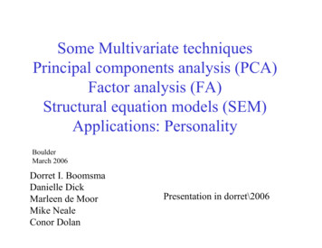
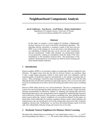
rank at most d. To achieve this, we apply the NCA learning algorithm to find the optimaltransformation A, and then we store only the projections of the training points yn Axn(as well as their labels). At test time, we classify a new point xtest by first computing itsprojection ytest Axtest and then doing KNN classification on ytest using the yn anda simple Euclidean metric. If d is relatively small (say less than 10), we can preprocessthe yn by building a KD-tree or a ball-tree to further increase the speed of search at testtime. The storage requirements of this method are O(dN ) Dd compared with O(DN )for KNN in the original input space.4Experiments in Metric Learning and Dimensionality ReductionWe have evaluated the NCA algorithm against standard distance metrics for KNN and othermethods for linear dimensionality reduction. In our experiments, we have used 6 data sets(5 from the UC Irvine repository). We compared the NCA transformation obtained fromoptimizing f (for square A) on the training set with the default Euclidean distance A I,1the “whitening” transformation , A Σ 2 (where Σ is the sample data covariance matrix), 1and the RCA [1] transformation A Σw 2 (where Σw is the average of the within-classcovariance matrices). We also investigated the behaviour of NCA when A is restricted tobe diagonal, allowing only axis aligned Mahalanobis measures.Figure 1 shows that the training and (more importantly) testing performance of NCA isconsistently the same as or better than that of other Mahalanobis distance measures forKNN, despite the relative simplicity of the NCA objective function and the fact that thedistance metric being learned is nothing more than a positive definite matrix A A.We have also investigated the use of linear dimensionality reduction using NCA (with nonsquare A) for visualization as well as reduced-complexity classification on several datasets.In figure 2 we show 4 examples of 2-D visualization. First, we generated a synthetic threedimensional dataset (shown in top row of figure 2) which consists of 5 classes (shown bydifferent colors). In two dimensions, the classes are distributed in concentric circles, whilethe third dimension is just Gaussian noise, uncorrelated with the other dimensions or theclass label. If the noise variance is large enough, the projection found by PCA is forcedto include the noise (as shown on the top left of figure 2). (A full rank Euclidean metricwould also be misled by this dimension.) The classes are not convex and cannot be linearly separated, hence the results obtained from LDA will be inappropriate (as shown infigure 2). In contrast, NCA adaptively finds the best projection without assuming any parametric structure in the low dimensional representation. We have also applied NCA to theUCI “wine” dataset, which consists of 178 points labeled into 3 classes and to a databaseof gray-scale images of faces consisting of 18 classes (each a separate individual) and 560dimensions (image size is 20 28). The face dataset consists of 1800 images (100 for eachperson). Finally, we applied our algorithm to a subset of the USPS dataset of handwrittendigit images, consisting of the first five digit classes (“one” through “five”). The grayscaleimages were downsampled to 8 8 pixel resolution resulting in 64 dimensions.As can be seen in figure 2 when a two-dimensional projection is used, the classes are consistently much better separated by the NCA transformation than by either PCA (which isunsupervised) or LDA (which has access to the class labels). Of course, the NCA transformation is still only a linear projection, just optimized with a cost function which explicitlyencourages local separation. To further quantify the projection results we can apply anearest-neighbor classification in the projected space. Using the same projection learnedat training time, we project the training set and all future test points and perform KNN inthe low-dimensional space using the Euclidean measure. The results under the PCA, LDA,LDA followed by RCA and NCA transformations (using K 1) appear in figure 1. TheNCA projection consistently gives superior performance in this highly constrained low-
distance metric learning trainingdistance metric learning 70.650.65NCAdiag diag NCARCAwhitenedEuclidean0.60.55housdigit0.5balrank 2 transformation training1iriswinehousdigitrank 2 transformation testing1NCALDA inehousdigitNCALDA ure 1: KNN classification accuracy (left train, right test) on UCI datasets balance, ionosphere, iris, wine and housing and on the USPS handwritten digits. Results are averagesover 40 realizations of splitting each dataset into training (70%) and testing (30%) subsets(for USPS 200 images for each of the 10 digit classes were used for training and 500 fortesting). Top panels show distance metric learning (square A) and bottom panels showlinear dimensionality reduction down to d 2.rank KNN setting. In summary, we have found that when labeled data is available, NCAperforms better both in terms of classification performance in the projected representationand in terms of visualization of class separation as compared to the standard methods ofPCA and LDA.5Extensions to Continuous Labels and Semi-Supervised LearningAlthough we have focused here on discrete classes, linear transformations and fully supervised learning, many extensions of this basic idea are possible. Clearly, a nonlineartransformation function A(·) could be learned using any architecture (such as a multilayerperceptron) trainable by gradient methods. Furthermore, it is possible to extend the classification framework presented above to the case of a real valued (continuous) supervisionsignal by defining the set of “correct matches” Ci for point i to be those points j havingsimilar (continuous) targets. This naturally leads to the idea of “soft matches”, in whichthe objective function becomes a sum over all pairs, each weighted by their agreement according to the targets. Learning under such an objective can still proceed even in settingswhere the targets are not explicitly provided as long as information identifying close pairs
PCALDANCAFigure 2: Dataset visualization results of PCA, LDA and NCA applied to (from top) the“concentric rings”, “wine”, “faces” and “digits” datasets. The data are reduced from theiroriginal dimensionalities (D 3,D 13,D 560,D 256 respectively) to the d 2 dimensionsshow.
Figure 3: The two dimensional outputs of the neural network on a set of test cases. On the left, eachpoint is shown using a line segment that has the same orientation as the input face. On the right, thesame points are shown again with the size of the circle representing the size of the face.is available. Such semi-supervised tasks often arise in domains with strong spatial or temporal continuity constraints on the supervision, e.g. in a video of a person’s face we mayassume that pose, and expression vary slowly in time even if no individual frames are everlabeled explicitly with numerical pose or expression values.To illustrate this, we generate pairs of faces in the following way: First we choose two facesat random from the FERET-B dataset (5000 isolated faces that have a standard orientationand scale). The first face is rotated by an angle uniformly distributed between 45o andscaled to have a height uniformly distributed between 25 and 35 pixels. The second face(which is of a different person) is given the same rotation and scaling but with Gaussiannoise of 1.22o and 1.5 pixels. The pair is given a weight, wab , which is the probabilitydensity of the added noise divided by its maximum possible value. We then trained a neuralnetwork with one hidden layer of 100 logistic units to map from the 35 35 pixel intensitiesof a face to a point, y, in a 2-D output space. Backpropagation was used to minimize thecost function in Eq. 8 which encourages the faces in a pair to be placed close together:!Xexp( ya yb 2 )Cost (8)wab log P2c,d exp( yc yd )pair(a,b)where c and d are indices over all of the faces, not just the onesthat form a pair. Four example faces are shown to the right; horizontally the pairs agree and vertically they do not. Figure 3 aboveshows that the feedforward neural network discovered polar coordinates without the user having to decide how to represent scaleand orientation in the output space.6Relationships to Other Methods and ConclusionsSeveral papers recently addressed the problem of learning Mahalanobis distance functionsgiven labeled data or at least side-information of the form of equivalence constraints. Tworelated methods are RCA [1] and a convex optimization based algorithm [7]. RCA isimplicitly assuming a Gaussian distribution for each class (so it can be described usingonly the first two moments of the class-conditional distribution). Xing et. al attempt tofind a transformation which minimizes all pairwise squared distances between points in the
same class; this implicitly assumes that classes form a single compact connected set. Forhighly multimodal class distributions this cost function will be severely penalized. Lowe[6]proposed a method similar to ours but used a more limited idea for learning a nearestneighbour distance metric. In his approach, the metric is constrained to be diagonal (aswell, it is somewhat redundantly parameterized), and the objective function corresponds tothe average squared error between the true class distribution and the predicted distribution,which is not entirely appropriate in a more probabilistic setting.In parallel there has been work on learning low rank transformations for fast classificationand visualization. The classic LDA algorithm[3] is optimal if all class distributions areGaussian with a single shared covariance; this assumption, however is rarely true. LDAalso suffers from a small sample size problem when dealing with high-dimensional datawhen the within-class scatter matrix is nearly singular[2]. Recent variants of LDA (e.g.[5], [2]) make the transformation more robust to outliers and to numerical instability whennot enough datapoints are available. (This problem does not exist in our method since thereis no need for a matrix inversion.)In general, there are two classes of regularization assumption that are common in linearmethods for classification. The first is a strong parametric assumption about the structure ofthe class distributions (typically enforcing connected or even convex structure); the secondis an assumption about the decision boundary (typically enforcing a hyperplane). Ourmethod makes neither of these assumptions, relying instead on the strong regularizationimposed by restricting ourselves to a linear transformation of the original inputs.Future research on the NCA model will investigate using local estimates of K as derivedfrom the entropy of the distributions pij ; the possible use of a stochastic classification ruleat test time; and more systematic comparisons between the objective functions f and g.To conclude, we have introduced a novel non-parametric learning method — NCA — thathandles the tasks of distance learning and dimensionality reduction in a unified manner.Although much recent effort has focused on non-linear methods, we feel that linear embedding has still not fully fulfilled its potential for either visualization or learning.AcknowledgmentsThanks to David Heckerman and Paul Viola for suggesting that we investigate the alternative cost g(A) and the case of diagonal A.References[1] A. Bar-Hillel, T. Hertz, N. Shental, and D. Weinshall. Learning distance functions using equivalence relation. In International Conference on Machine Learning, 2003.[2] L. Chen, H. Liao, M. Ko, J. Lin, and G. Yu. A new lda-based face recognition system which cansolve the small sample size problem. In Pattern Recognition, pages 1713–1726, 2000.[3] R. A. Fisher. The use of multiple measurements in taxonomic problems. In Annual of Eugenic,pages 179–188, 1936.[4] J. Friedman, J.bentley, and R. Finkel. An algorithm for finding best matches in logarithmicexpected time. In ACM, 1977.[5] Y. Koren and L. Carmel. Robust linear dimensionality reduction. In IEEE Trans. Vis. and Comp.Graph., pages 459–470, 2004.[6] D. Lowe. Similarity metric learning for a variable kernel classifier. In Neural Computation,pages 72–85, 1995.[7] E.P. Xing, A. Y. Ng, M.I. Jordan, and S. Russell. Distance learning metric. In Proc. of NeuralInformation Processing Systems, 2003.
Neighbourhood Components Analysis Jacob Goldberger, Sam Roweis, Geoff Hinton, Ruslan Salakhutdinov Department of Computer Science, University of Toronto {jacob,roweis,hinton,rsalakhu}@cs.toronto.edu Abstract In this paper we propose a novel method for learning a Mahalanobis distance measure to be used in the KNN classification algorit hm. The