WIXLIB

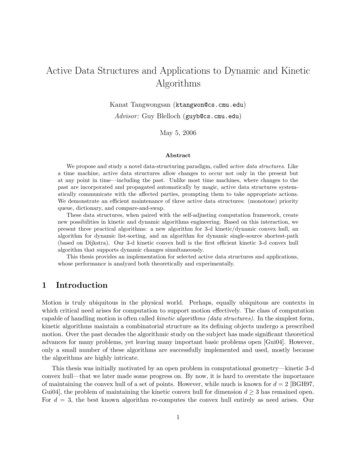
probability-density function on bit strings {0, 1} . For all n N, define d(n) max Eφ [δtr tr(P, I), tr(P, I 0 ) ].(I,I 0 ) nWe say that P is expected S-stable for and φ if d(·) S.Note that expected O(f (·)) stable, Ω(f (·)) stable, and Θ(f (·)) are all valid uses of the stabilitynotation. Worst-case stability is defined by dropping the expectation from the definition.We define monotonicity of a program as in Acar et al. [ABH 04] and state the following theorems, which are useful in the sequel.Theorem 4 (Stability Theorem [ABH 04]) If an algorithm is O(f (n))-stable for a class ofinput changes , then each operation will take at most O(f (n) log n).However, if the discrepancy set has a bounded size, then each operation can be performed inO(f (n)).Theorem 5 (Triangle Inequality for Change Propagation) Let P be a monotone programwith respect to the class of changes 1 and 2 . Suppose that P is O(f (n)) and O(g(n)) stablefor 1 and 2 , respectively, for some measure n. P is also monotone with respect to the class ofchanges ( 1 2 ) obtained by composing 1 and 2 , then P is O(f (n) g(n)) stable for 1 o 2 .A proof of this theorem is supplied in the appendix.3Active Data StructuresWe introduce a new data structuring paradigm, called active data structures. Akin to the retroactivedata structures [DIL04], active data structures allow the data-structure operations to take placenot only in the present but also in the past. When an operation is performed, an active datastructure, in addition to fixing the internal states, identifies which other operations take on newresulting values and notifies them to adjust to the changes. This capability has an importantsoftware-engineering benefit: composibility.Consider a database for bank accounts at a financial company. Suppose that, at 12pm, we discover that an important transaction performed earlier at 9am was erroneous, and we need to correctit. Most traditional systems would need to rollback the transactions to 9am, where we then correctthe record and recommit subsequent transactions. Using a retroactive data structure [DIL04], onewould, in one-step, magically tell the data structure to correct the operation performed at 9am andrejoice. However, it is often inadequate to make corrections only internally to the data structure.In this example, suppose further that a banker performed a query at 10am, whose result is used inan investment plan recorded to the database at 11am. It is critical to notify the person performingthe query at 10am to consider the new value and update the plan.Comparison to Persistent Data Structures. While persistent data structures and activedata structures both consider the notion of time, they are inherently different—both in terms of4

9AMDiscover the Erroraction6AMBobPlaDe nnincis gion.ErroneousTransTransactions12PMTimeFigure 1: The ability to change the past can be important. Many real-world applications alsorequire composibility.their functionalities and the underlying ideas. A persistent data structure is characterized by theability to access any past versions of the data structure. In terms of changes, the simplest form ofpersistency, called partial persistency, allows changes only in the present and queries for any pastversions. A fully persistent data structure, although allowing changes to occur in the past, does notpropagate the effects of the changes to the present. Instead, it creates a new branch in the versiontree, as illustrated in Figure 2.An action in the past causesthe version tree to branches offTime/VersionsFigure 2: Changes to the past in a fully persistent data structure.Comparison to Retroactive Data Structures. Even though retroactive data structuresand active data structures appear highly related as they both allow changes to occur in the presentand in the past, they significantly differ. In a retroactive data structure, operations performed onthe data structure are reflected only internally. An outside party who retrieves some data fromthe data structure has no way of knowing that the data is outdated. This is illustrated by thebank-database example mentioned earlier. In an active data structure, the affected parties will becommunicated.The Notion of Time and Maintaining a Virtual Time Line. In order for the notionof time to make sense, we assume a time line is somehow maintained so that each action can betimestamped with a unique time. In practice, a virtual time line can be maintained efficiently usingan order-maintenance data structure [DS87, BCD 02]. These order-maintenance data structurescan simulate a virtual time line in amortized O(1). In what follows, we assume a time line is theset of non-negative reals (R {0}), and each time-stamp is a unique real number t R {0}.5

3.1Defining Active Data StructuresWe introduce vocabularies for discussing about active data structures. For comparison, considera usual data structure D with operations operation1 , operation2 , operation3 , . . . , operationk . Ina usual data structure, all operations are performed at the present time, altering the state of thedata structure and destroying the previous version. An active data structure enables performing(or undoing) the operations at any time. We define 3 meta-operations that characterize active datastructures as follows: The meta-operation perform(“operationi (·)”, t) will perform the operation operationi at thetime t. If operationi (·) returns a value ri , then the meta-operation returns the value ri . The meta-operation undo(t) causes an undo of the operation at the time t. The meta-operation update(t) informs the data structure to “synchronize” up to time t. Thisoperation will become more clear once it appears in context.In addition, we assume the existence of a discrepancy set; this is maintained either by the datastructure itself or as a part of another framework (cf. self-adjusting computation). The discrepancyset is a list of entities (e.g., a data structure operation, human interaction) that need to take someactions, because the information the entity receives has changed since the last communication.In the banking example, an entity could be Bob, who needs to know that the information heobtained is now outdated. The idea of the discrepancy set is that, as soon as an entity is identify asdiscrepant, it is inserted to the set. The entries of the discrepancy set are removed and processedin an increasing order of time until the set becomes empty, at which point the data structure isfully synchronized with the current reality. In practice, the discrepancy set can be maintained in apriority queue.3.2Active Compare-and-SwapWe begin our discussion of active data structures by introducing a basic data structure, calledcompare-and-swap. Despite its fancy name, a compare-and-swap data structure is a plain-old datastructure commonly found in algorithms. Without the notion of time, the data structure has onlyone operation, touch, and maintains a boolean variable b, whose value is initially false. If thedata structure is touched, the variable b changes to true and remains true for the rest of the time.The touch operation returns the current status of b and subsequently updates the value of b.This simple data structure appears extensively as a tiny component of bigger data structuresand algorithms. It is, for example, a part of the bit vector in many implementations of depth-firstsearch, indicating whether or not a node has been visited. The name compare-and-swap emergesfrom the actions it performs. In many applications, once b is set to true no more operation will beperformed on the corresponding object.Similar to a regular compare-and-swap, an active compare-and-swap has only one operation,touch, which can be both performed and undone at an arbitrary time. We formally describe anactive compare-and-swap as follows. This description outlines the general characteristics of the datastructure; an efficient compare-and-swap will be discussed later. Let S be the set of times at whichthe data structure is touched. Initially S is an empty set. For the purpose of this presentation,6

think of S as a global variable, which is updated as operations are performed on the data structure.Like any active data structures, an active compare-and-swap supports the following: Support for the meta-operation perform. The operation perform(“touch”, t)—performinga touch at time t—maintains the following invariants. The return value of the operation isfalse if and only if t min S, with min . After the operation, the set S is augmentedto contain t. That is, S : S {t}. Support for the meta-operation undo. The operation undo(t)—undoes a touch at timet—updates the set S as S : S \ {t}. Support for the meta-operation update. The operation checks if the return value of thetouch operation at that time has changed. If the value is changed, it tells the discrepancyset that the person who retrieves this information is discrepant.We point out that both of these operations may alter the return values of some other touchoperations. An active compare-and-swap data structure has to be able to identify these operationsand re-synchronize accordingly.Efficient Compare-and-Swap. In the remaining of this section, we describe an efficientmaintenance of an active compare-and-swap data structure. For ease, we maintain the set S in abalanced search tree (e.g. red-black tree). Maintaining S as a combination of a priority queue and ahash table is an equally viable option and will yield the same asymptotic bounds. The needed basicset operations, including finding the minimum, can be trivially performed on a balanced binarysearch tree in O(log S ).As mentioned earlier, an operation can affect the return values of other operations. We observethat, in this particular data structure, an operation can affect at most 1 other operation. Performinga touch at the time t will cause a side-effect if and only if t min S, in which case the return valueof the old minimum is altered. An undo of the operation at time t causes a side-effect if only if t isthe current minimum of S, in which case the return value of the second minimum of S is changed.We note that the number of active touch’s T is same as S throughout, and establish the followingtheorem.Theorem 6 An active compare-and-swap can be maintained in O(log T ) for all operations, whereT is the number of active touch’s. We say that a touch operation is active if it has been performedand has not been undone.3.3Active Monotone Priority QueueWe consider the problem of maintaining an active monotone priority queue. The monotone assumption greatly simplifies the problem but suffices for many applications; at the end of this section, wediscuss problems with generalizing this to an unrestricted priority queue. Without loss of generality,we assume that the keys (a.k.a. priorities) are positive real numbers (R ) Informally, a monotonepriority queue disallows inserting a key smaller than latest minimum removed by the deleteminoperation. We precisely formulate the problem and formally state this assumption below.7

Let DM be the set of times at which a deletemin occurs. Let INS be the set of ordered pairs ofthe form (k, t). Each entry (k, t) INS denotes the insertion point of the key k at the time t. Weassume for simplicity that no duplicate keys are inserted.Definition 7 Let PQ(t) be the set containing all keys inserted on or before the time t that have notbeen removed by the deletemin operation. The set PQ(t) is a hypothetical snapshot of the priorityqueue at time t. Initially PQ(0) .Definition 8 (Monotone Assumption) Let f (t) : min PQ(t). A priority queue is said to bemonotone if for all t1 , t2 DM with t1 t2 , f (t1 ) f (t2 ).Our priority queue supports two operations: insert and deletemin. The problem of maintainingactive priority queue has the following characteristics: Support for the meta-operation perform. The operation perform(“insert(k)”, t)—performingan insertion of the key k at time t—causes the following changes: INS : INS {(k, t)}. Thisoperation returns nothing.The operation perform(“deleteMin”, t) calculates the return value as min PQ(t) and altersDM to DM {t}. We note that this description does not describe how to efficiently maintainsuch a structure. Support for the meta-operation undo. The operation undo(t) for an insert operationsimply removes the corresponding ( , t) from INS. Similarly, the operation undo(t) for andeleteMin operation removes t from DM.********Efficient Monotone Priority Queue. We give a solution to the problem of efficiently maintaining an active monotone priority queue. Our data structure maintains 2 balanced binary searchtrees (e.g. red-black, AVL tree): TDM and TINS , corresponding to the sets DM and INS, respectively.The tree TDM is naturally ordered by time. The other tree TINS is indexed by first the key thenthe the time. That is, (k1 , t1 ) (k2 , t2 ) if and only if (k1 k2 ) or ((k1 k2 ) (t1 t2 )). Eachdeletemin—a node of TDM —is linked with a node of TINS whose key is the result of that deletemin.Each node of TINS is vice versa linked with its corresponding deletemin when applicable.As an active data structure, our active priority queue is responsible for identifying the operationswhose return values are affected, in addition to maintaining the invariants stated earlier. Theproblem of identifying the affected operations are discussed later. We will now focus on the problemof the maintaining the aforementioned invariants: The operation perform(“insert(k)”, t) results in an insertion of the key (k, t) to the tree TINS .The undo operation for an insert is handled vice versa by removing the key (k, t) from thetree. The operation perform(“deletemin”, t) adds an entry t to the tree TDM , and its undo operationremoves t from TDM . The return value of perform(“deletemin”, t) is derived as follows.8

Compute t : max{t0 DM : t0 t}, with max . If t , report the minimumkey in TINS . Otherwise, query TDM for the corresponding value the delete; call this valuek . Make another query to TINS for k : min{k0 Keys(INS) : k0 k }, where Keys(INS)contains all the keys existed in INS. Report k . It is trivial to fix the cross-links between thetwo trees.********keyskeysA Ray-shooting Game and Discrepancy Detection. We introduce a “ray-shooting” game,which illustrates the processing of finding the affected operations. Every sequence of operationsin a retroactive data structure can be visually represented as follows. Consider a two-dimensionaldiagram, whose horizontal axis represents time and vertical axis represents the keys of the elementsof interest. Recall that each key is a positive real number. An example of such diagram is shown inFigure 3 (left). Each horizontal line represents the lifespan of its corresponding key. It originateswhere the key is inserted and extends to the right either indefinitely if it is never removed bya deletemin or until it vanishes at the time when removed by a deletemin. Each vertical linerepresents a deletemin operation. It always originates from the horizontal axis and extends upwardup to the height of the key that the deletemin operation returns.ABttFigure 3: Visualizing an Active Priority Queue using Ray-shootingThe task of identifying the affected operations can thought of as two cases of ray shooting:rightward and upward. Inserting a key k at time t is equivalent to ray-shooting rightward fromthe point (t, k), as depicted in the point A in Figure 3 (right). We say that a line segment isoccupied if it meets with another line segment of a different orientation. Removing a key will“free” a vertical segment; such a segment is affected. A new return value for that deletemin canbe calculated by performing an upward ray-shooting as depicted at point B in Figure 3 (right).The two other operations can be handled similarly. With the monotonicity assumption, these rayshooting operations can be efficiently performed on the two trees in O(log T ), where T is the totalnumber of active operations on the data structure. As before, an operation is active if it has beenperformed but not undone.Theorem 9 An active monotone priority queue can be maintained in an amortized O(log T ) for9

all operations, where T is the number of active operations.We point out that an active full priority queue is much more involved, as it demands a pointlocation data structure. In particular, the trick that allows us to compute the current minimumwill not generalize, because it relies on the monotonicity assumption. We conclude the discussionof active priority queues by listing a number of applications that admit the monotone assumption.In Dijkstra, the distance of the nodes as maintained in a priority is monotone. The same is truefor Prim’s algorithm for computing a minimum spanning tree. A monotone priority queue can alsobe used to ensure that certain operations are performed in order. Two real-world applications thatillustrate such use are discussed in a subsequent section.3.4Active DictionaryA dictionary data structure supports three basic operations: insert(key, data), lookup(key), anddelete(key). Let U be the universe of keys the dictionary supports. We assume that either U istotally ordered or there exists a universal hash function h : U [m] for m N. This assumptionis realistic and allows an easy maintenance of an active dictionary.Like other active data structures we discuss, an active dictionary has the same three operations—insert, lookup, and delete—wrapped in the meta-operations perform, undo, and update. In order tosupport these operations, an active dictionary maintains the following structures internally. Eachkey k U is associated with three sets: INS(k), DEL(k), QUERY(k). First, the set INS(k) keepstrack of all insert operations performed on the key k. Entries of this set take the form (t, d), wheret denotes the time and d is the data associated with that insertion. Second, the set DEL(k) containsthe times at which delete operations are performed on the key k. Finally, the set QUERY(k) recordsthe times at which queries to the key k take place. These sets can be trivially maintained for therequired data structure operations.Efficient Active Dictionary. The problem of maintaining an active dictionary can be reducedto a simpler problem in the following manner. When an operation about a key k is received, the datastructure refers to the three sets—INS(k), DEL(k), and QUERY(k)—on which actions are performed.We note that it suffices to consider only these three sets to support any operations regarding thekey k. Because of our assumption about the universe of keys, locating the corresponding three setscan be easily accomplished by a hash table or a (balanced) binary search tree.We now turn our focus to maintaining the three sets for each key and how they can be usedto support all dictionary operations. Therefore, when the context is clear, we drop the mention ofkey. Consider Figure 4. The sets INS and DEL combine to a set of intervals in which the key ispresent in the dictionary. Formally, letd (t) : {t0 DEL : t0 t}andIV : {(α, inf d (α)) : α TIME(INS)} ,where (α, β) denotes the open-interval from α to β (exclusive), and inf(·) is the infimum. We notethat at most one interval is unbounded, corresponding to an insertion which is never deleted. Alookup at time t finds the key (and its corresponding data) if and only t lies in one of the intervals10

QINSDEL)(()Queries()IntervalsFigure 4: The sets INS and DEL combine to a set of intervals in which the key is present in thedictionary.of IV. If a lookup at time t satisfies t (α, β) for (α, β) IV, then the lookup operation finds thekey, where the data is the data of the insertion at time α.Let Tk be the number of operations on which the key k. The sets INS, DEL, and QUERY canbe trivially represented with balanced binary search trees, where needed operations take at mostO(log Tk ) time.Theorem 10 For a fixed key k, an active dictionary can be maintained in an amortized O(log Tk )for all operations, where Tk is the number of active operations on the key k. Let n the total numberof keys. Assume that a balanced binary search tree is used to locate the right triple of sets; then,every operation in the active dictionary runs in O(log n log Tk ).4Dynamic Heap SortWe demonstrate how an active data structure can be used in conjunction with the self-adjusting library to implement a dynamic algorithm. We consider a simple problem of maintaini

data structures can help simplify and improve many dynamic algorithms. Section 4 illustrates a simple use of active data structures to the dynamic list-sorting problem. In Section 5, we describe a new practical algorithm for maintaining the kinetic 3-d convex hull based on active data structures. This algorithm greatly improves on the naive method.