WIXLIB

Lecture 9[DR. MUHAMMAD NAEEM ARBAB]Lecture # 9Solved Examples of Plotting Root LocusDear Student this lecture is based on the technique of sketching the root locus as described inLecture 8. Remember that for plotting the root locus, the open-loop transfer function is required.Here three examples are considered. In Example 1, the open-loop transfer function is given soeverything is crystal clear; open-loop poles and open-loop zeros are found directly, which arenecessary to start drawing the root locus. In Example 2, the closed-loop transfer function isgiven, from which the open-loop transfer function is obtained, which can be factorized forobtaining open-loop poles and zeros. So things are not directly. Example 3, deals with thesituation when we encounter complex open-loop poles and zeros. In this case a few conventionalparameters; such as breakaway point and break-in points and sometimes jω-crossing points aremissing. However, two new parameters are introduced; angle of departure from complex openloop pole (replacing the breakaway point) and angle of arrival at a complex open-loop zero(replacing the break-in point).K ( s 1)s( s 2)( s 3)Solution: The system’s open-loop poles are 0, –2 and –3 and open-loop zero is: –1, and there aretwo zeros lying at infinity.Example 1: Plot the root locus for a system whose open-loop transfer function is:Number of loci: N number of open-loop poles 3Real-axis loci: From the location of open-loop poles and zeros in the s-plane, the real-axis lociwill exist between 0 and –1 and between –2 and –3. p zCenter of asymptotes: C Angles of asymptotes:(2k 1)1800 Cp zip zi 0 2 3 0 2.53 1For k 0; C 900 , for k 1; C 2700 . The angles are repeated in the same sequence for k 2, 3, Breakaway point:1111 b 1 b b 2 b 3From which: b 3 4 b 2 5 b 3 01 Control System Engineering

Lecture 9This gives:[DR. MUHAMMAD NAEEM ARBAB] b 2.465Break-in point: There is no break-in point since there is no real axis loci between two open-loopzeros. However, there are two open-loop zeros lying at infinity, and the root locus will tend tomove to infinity from breakaway point to search for their zeros lying at infinity.jω-crossing: There is no jω-crossing since the root locus will depart from the real-axis at 90o and270o. The complete root locus is shown in Figure (1).Figure 1Example 2: Draw the root locus of a control system whose closed-loop transfer function is:K.32s 6s 9s KSolution: The given system can be converted to a unity feedback configuration by consideringthe given transfer function and manipulating it as:K /( s 3 6s 2 9s)G( s) 321 K /( s 6s 9s) 1 H (s)G(s)2 Control System Engineering

Lecture 9[DR. MUHAMMAD NAEEM ARBAB]G(s) H (s) Thus:KK s(s 6s 9) s(s 3) 22The system poles are: 0, –3 and –3. There are three zeros lying at infinity.Number of loci: N number of open-loop poles 3.Real-axis loci: From the location of open-loop poles, the real-axis loci will exist between 0 and–3 and from –3 to – .Center of asymptotes: C Angles of asymptotes: C pi z ip z 0 3 3 0 23 0(2k 1)1800 (2k 1)1800 p z3 0For k 0; C 600 , for k 1; C 1800 and for k 2; C 3000 . The angles are repeated inthe same sequence for k 3, 4, 5, Breakaway point: From the characteristic equation: s 3 6s 2 9s K we have:dK 3s 2 12s 9 0dsThis yield:3 b 12 b 9 02Which give real roots; –1 and –3. The real root: –1 is within the real-axis loci between 0 and –3,therefore the real root; b 1 is the breakaway point.Break-in point: There is no break-in point since the root locus will tend to move to infinity frombreakaway point to search for zeros lying at infinity.jω-crossing: The jω-crossing point can be obtained by considering the characteristic polynomialof the closed-loop transfer function: s 3 6s 2 9s K from which the Routh table is formedbelow:s319s26K3 Control System Engineering

Lecture 9[DR. MUHAMMAD NAEEM ARBAB]s154 K60s0K0Forcing the term of the first column of s1 row to be zero, we can form an auxiliary equation ofthe preceding even row. Thus for K 54, we will have an all-zero row. The auxiliary equation ofthe preceding row of even power of s is then: 6s 2 54 0 , which yields:s j3Which are the required points of jω-crossing. The complete root locus is shown in Figure (2).Figure 24 Control System Engineering

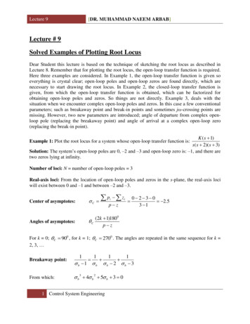
Lecture 9[DR. MUHAMMAD NAEEM ARBAB]Example 3: Plot the root locus of the unity feedback system whose forward transfer function isK (s 2 4s 13)G(s) given as:.(s 4)( s 2 2s 5)Solution: The open-loop transfer function of the given unity feedback system is:G( s) H ( s) K (s 2 4s 13)(s 4)( s 2 2s 5)The open-loop transfer function can be conveniently factorized as:G( s) H ( s) K (s 2 j3)( s 2 j3)(s 4)( s 1 j 2)( s 1 j 2)The system poles are: –4, and 1 j 2 . The complex zeros are: 2 j3 and 2 j3 . There is azero lying at infinity.Number of loci: Number of loci (N) number of open-loop poles 3Real-axis loci: From the position of open-loop poles and zeros, the real-axis loci exist at –4 andmoves towards negative infinity direction in search of its zero lying at infinity. Since the realaxis loci tends to move towards infinity in search of the zero lying at infinity and the loci startingfrom the complex poles will terminate on the complex zeros, therefore there is no breakaway andbreak-in point on the real-axis. Thus the centre and angles of asymptotes will not exist. The rootlocus in the s-plane will terminate on the complex zeros therefore there will be no jω-crossingpoint.Angle of departure at complex poles: Considering a complex pole s 1 j 2 , the angle ofdeparture θD can be determined by ignoring the angle contribution from the factor of the complexpole considered and then finding the angle contribution of the remaining poles and zeros at:s 1 j 2 . This angle contribution is then: K[G(s) H (s)] / . Where the function: K[G(s) H (s)]/ is the open-loop transfer function in which the angle contribution of the complexpole of interest has been ignored. Thus:K[G(s) H ( s)] / K (1 j5)(1 j1)(3 j 2)( j 4) 78.7 0 450 90000 33.7 90Therefore: K[G(s) H (s)] / Therefore: D 1800 K[G(s) H (s)]/ 1800 900 9005 Control System Engineering

Lecture 9[DR. MUHAMMAD NAEEM ARBAB]Angle of arrival at a complex zero: Since in this example there are two complex zeros, the locifrom the complex poles will terminate on the complex zeros. The angle of arrival at a complexzero ( s 2 j3 ), can be determined from the given open-loop transfer function by ignoring theangle contribution from the zero of interest ( s 2 j3 ). The open-loop transfer function inwhich the factor of the considered zero is ignored will be: K[G(s) H (s)] // . The anglecontribution of K[G(s) H (s)] // is the argument of this function, which is obtained as follows:K[G(s) H ( s)] // K ( s 2 j3)(s 4)( s 1 j 2)( s 1 j 2)At s 2 j3 , the function will be:K[G(s) H (s)] // K ( j 6)(2 j3)( 1 j5)( 1 j1) 900 K[G(s) H (s)] 202.6 0000 56.3 101.3 135//Therefore the angle of arrival at the complex pole of interest is: A 180o K[G(s) H (s)]// 1800 202.6 0 382.60 or 22.60Since the function contains two complex poles and two complex zeros in the LHP, the loci fromthe complex poles will terminate on the corresponding complex zeros, therefore there will be nojω-crossing point. The other zero is lying at infinity and the loci from the real-axis pole –4 willmove to infinity in search of the zero lying at infinity. The complete root locus is shown inFigure (3).6 Control System Engineering

Lecture 9[DR. MUHAMMAD NAEEM ARBAB]Figure 37 Control System Engineering

3 Control System Engineering Thus: 2 6 9( 3) 2 ( ) ( ) s K K G s H s The system poles are: 0, -3 and -3. There are three zeros lying at infinity. Number of loci: N number of open-loop poles 3. Real-axis loci: From the location of open-loop poles, the real-axis loci will exist between 0 and -3 and from -3 to - . Center of .