Transcription
The Stata Journal, 2002, 3, pp 316-327The Clustergram: A graph for visualizing hierarchical andnon-hierarchical cluster analysesMatthias SchonlauRANDAbstractIn hierarchical cluster analysis dendrogram graphs are used to visualize how clusters areformed. I propose an alternative graph named “clustergram” to examine how clustermembers are assigned to clusters as the number of clusters increases. This graph is usefulin exploratory analysis for non-hierarchical clustering algorithms like k-means and forhierarchical cluster algorithms when the number of observations is large enough to makedendrograms impractical. I present the Stata code and give two examples.Key WordsDendrogram, tree, clustering, non-hierarchical, large data, asbestos1. IntroductionThe Academic Press Dictionary of Science and Technology defines a dendrogram asfollows:dendrogram Biology. a branching diagram used to show relationships between membersof a group; a family tree with the oldest common ancestor at the base, and branches forvarious divisions of lineage.1
In cluster analysis a dendrogram ([R] cluster dendrogram and, for example, Everitt andDunn, 1991, Johnson and Wichern, 1988) is a tree graph that can be used to examinehow clusters are formed in hierarchical cluster analysis ([R] cluster singlelinkage, [R]cluster completelinkage, [R] cluster averagelinkage). Figure 1 gives an example of adendrogram with 75 observations. Each leaf represents an individual observation. Theleaves are spaced evenly along the horizontal axis. The vertical axis indicates a distanceor dissimilarity measure. The height of a node represents the distance of the two clustersthat the node joins. The graph is used to visualize how clusters are formed. For example,if the maximal distance on the y axis is set to 40, then three clusters are formed becausey 40 intersects the tree three times.7060L2 dissimilarity measure504030201001103225146184812715920162122411 923251317263241434842 7 96751746959616675 256 3587254736568Figure 1 A dendrogram for 75 observations2
Dendrograms have two limitations: (1) because each observation must be displayed as aleaf they can only be used for a small number of observations. Stata 7 allows up to 100observations. As Figure 1 shows, even with 75 observations it is difficult to distinguishindividual leaves. (2) The vertical axis represents the level of the criterion at which anytwo clusters can be joined. Successive joining of clusters implies a hierarchical structure,meaning that dendrograms are only suitable for hierarchical cluster analysis.For large numbers of observations hierarchical cluster algorithms can be too timeconsuming. The computational complexity of the three popular linkage methods is oforder O(n2), whereas the most popular non-hierarchical cluster algorithm, k-means ([R]cluster kmeans, MacQueen, 1967), is only of the order O(kn) where k is the number ofclusters and n the number of observations (Hand et al., 2001). Therefore k-means, a nonhierarchical method, is emerging as a popular choice in the data mining community.I propose a graph that examines how cluster members are assigned to clusters as thenumber of clusters changes. In this way it is similar to the dendrogram. Unlike thedendrogram this graph can be used for non-hierarchical clustering algorithms also. I callthis graph a clustergram.The outline of the remainder of this paper is as follows: Section 2 and 3 contain syntaxand options of the Stata command clustergram, respectively. Section 4 explains how theclustergram is computed by means of an example related to asbestos lawsuits. The3
example also illustrates the use of the clustergram command. Section 5 contains a secondexample: Fisher’s famous Iris data. Section 6 concludes with some discussion.2. Syntaxclustergram varlist [if exp] [in range] , CLuster(clustervarlist)[ FRaction(#) fill graph options ]The variables specifying the cluster assignments must be supplied. I illustrate this in anexample below.3. Optionsclustervarlist specifies the variables containing cluster assignments, aspreviously produced by cluster.More precisely, they usuallysuccessively specify assignm ents to 1, 2, .clusters.Typically they will be named something like cluster1 -clustermax,where max is the maximum number of clusters identified.It ispossible to specify assignments other than to 1,2, . clusters(e.g. omitting the first few cluste rs, or in reverse order). Awarning will be displayed in this case. This option is required.fraction()specifies a fudge factor controlling the width of linesegments and is typically modified to reduce visual clutter.Therelative width of any two lin e segments is not affected. Thevalue should be between 0 and 1. The default is 0.2.4
fill specifies that individual graph segments are to be filled (solid).By default only the outline of each segment is drawn.graph options are options of graph, twowa y other than symbol() andconnect(). The defaults include ylabels showing three (rounded)levels and gap(5).4. Description and the Asbestos ExampleA huge number of lawsuits concerning asbestos-related personal injuries have been filedin the United States. One interesting question is: can companies be clustered into groupson the basis of how many lawsuits were filed against them? The data consist of thenumber of asbestos suits filed against 178 companies in the United States from 1970through 2000. Figure 2 shows a plot of the log base 10 of the number of asbestos suitsover time for each of the 178 companies. Few asbestos lawsuits were filed in the earlyyears. By 1990 some companies were subject to 10,000 asbestos related lawsuits in asingle year. I separate the number of asbestos suits by year to create 31 variables for thecluster algorithm. Each variable consists of the log base 10 of the number of suits thatwere filed against a company in a year.5
5log10(asbestos suits filed)432101970197519801985year199019952000Figure 2: Plot of the log base 10 number of asbestos suits over time for each of the 178companiesA principal component analysis of the covariance matrix of these 31 variables shows thatthe first principal component captures 82% and the second principal component 7% ofthe variation. The first principal component consists of a weighted average of allvariables with larger weights attributed to years with more lawsuits (approximately 19782000). Clearly, it is an overall measure of the number of lawsuits. The second principalcomponent consists of a contrast between variables corresponding to 1978-1992 andthose corresponding to 1993-2000. This component captures whether the number oflawsuits continued to increase, stagnate or decrease during this years. Figure 3 shows ascatter plot of the first two principal components. The cluster at the bottom consists ofcompanies with none or few lawsuits.6
nt2456789Figure 3: Scatter plot of the first two principal componentsIn preparation for constructing the clustergram, one needs to run the chosen clusteralgorithm multiple times; each time specifying a different number of clusters (e.g. 1through 20). One can create 20 cluster variables named “cluster1” through “cluster20”using the k-means clustering algorithm in Stata as follows:for num 1/20: cluster kmeans log1970-log2000, k(X) L1 name("clusterX")These variables are needed as inputs for the clustergram. The clustergram is constructedas follows: For each cluster within each cluster analysis, compute the mean over allcluster variables and over all observations in that cluster. For example, for x 2 clusterscompute two cluster means. For each cluster, plot the cluster mean versus the number of7
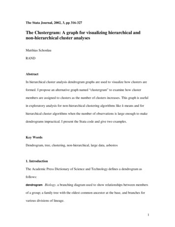
clusters. Connect cluster means of consecutive cluster analyses with parallelograms. Thewidth of each parallelogram indicates how many observations from a cluster wereassigned to a cluster in the following cluster analysis.Figure 4 illustrates this. Initially, all observations form a single cluster. This cluster issplit into two clusters. Since the lower parallelogram is much thicker then the upper one,there are many more observations that falling into the lower cluster. These two clustersare then split into three clusters. A new cluster is formed in the middle that draws someobservations that were previously classified in the lower cluster, and some that werepreviously classified in the higher cluster. Because the new cluster is formed fromobservations of more than one previous clusters (i.e. has more than one parent) this is anon-hierarchical split. The vertical axis refers to the log base 10 of the average number oflawsuits filed against a company. Therefore “higher” or “lower” clusters refer to clusterswith companies that on average have a larger or smaller number of lawsuits.8
2.5Cluster mean21.51.5012Number of clusters3Figure 4: A clustergram for 1–3 clusters. The cluster assignments stem from the kmeans algorithm.To avoid visual clutter the width of all parallelograms or graph segments can becontrolled through a fudge factor. This factor by default is 0.2 and can optionally be setby the user. The amount should be chosen large enough that clusters of various sizes canbe distinguished and small enough that there is not too much visual clutter.Using the syntax introduced in Section 2, the clustergram with up to 20 different clusterscan be obtained as follows:clustergram log1970-log2000, cluster(cluster1 -cluster20)fraction(0.1) xlab(1 2 to 20) ylab(0 0.5 to 3.5) fill9
3.53Cluster mean2.521.51.50123456789 10 11 12 13 14 15 16 17 18 19 20Number of clustersFigure 5: Clustergram with up to 20 clusters. The k-means cluster algorithm was used.Figure 5 displays the resulting clustergram for up to 20 clusters. We see that thecompanies initially split into two clusters of unequal size. The cluster with the lowestmean remains the largest cluster by far for all cluster sizes. One can also identifyhierarchical splits. A split is a hierarchical split when a cluster has only one parent orpredecessor. The split from 3 to 4 clusters is almost hierarchical (it is not strictlyhierarchical because a single company joins from the bottom cluster). Also, there are anumber of individual companies that appear to be hard to classify because they switchclusters.10
At 8 and 19 clusters the two clusters at the top merge and then de-merge again. Thishighlights a weakness of the k-means algorithm. For some starting values the algorithmmay not find the best solution. The clustergram in this case is able to identify theinstability for this data set.Figure 6 shows a clustergram for a hierarchical, average linkage cluster analysis. Thesewere obtained using the following Stata commands:cluster averagelinkage log1970 -log2000, L1 name("clusX")for num 1/20: cluster gen clusterX group(X)3.53Cluster mean2.521.51.50123456789 10 11 12 13 14 15 16 17 18 19 20Number of clustersFigure 6: A clustergram for the “average linkage” (hierarchical) cluster analysis.11
Because of the hierarchical nature of the algorithm, once a cluster is split off it cannotlater join with other clusters later on. Qualitatively, Figure 5 and Figure 6 convey thesame picture. Again, the bottom cluster has by far the most members, and the other twoor three major streams of clusters appear at roughly the same time with a very similarmean.In Figure 7 we see a clustergram for a hierarchical, single linkage cluster analysis. Mostclusters are formed by splitting a single company off the largest cluster. When the 11thcluster is formed the largest cluster shifts visibly downward. Unlike most of the previousnew clusters the 11th cluster has more than one member and its cluster mean of about 2.5is relatively large. The re-assignment of these companies to the 11th cluster causes themean of the largest cluster to drop visibly. If our goal is to identify several non-trivialclusters, this cluster algorithm does not suit this purpose. Figure 7 conveys thisinformation instantly.12
3.53Cluster mean2.521.51.50123456789 10 11 12 13 14 15 16 17 18 19 20Number of clustersFigure 7: A clustergram for the “single linkage” (hierarchical) cluster analysis.Of course, the ultimate decision of the number of clusters is always somewhat arbitraryand should be based on subject matter expertise, the criterion that measures within-clusterhomogeneity as well as insight gained from the clustergrams. It is re-assuring thatk-means and the algorithm “average linkage” lead to qualitatively similar results.5. Iris DataFisher’s Iris data (Fisher, 1938) consists of four variables: length and width of sepal andpetal of Iris. It is known that there are three different species of Iris, namely Iris setosa,Iris versicolor, and Iris virginica. It is of interest whether one can distinguish thesespecies based on these four variables. Figure 8 shows a scatter plot of petal length andwidth. This scatter plot best shows how the three species are separated. One species is13
relatively easy to distinguish from the other two; distinguishing between the other two isharder. Because the data consist of 150 observations a full dendrogram cannot be drawn.703333333petal length in 11111111111511015petal width in mm.2025Figure 8: Scatter plot of petal width and petal length of the Iris data. Different plottingsymbols indicate different species: (1) Iris setosa, (2) Iris versicolor, (3) Iris virginicaFigure 9 shows clustergrams for the k-means algorithm and the three linkage algorithmsfor cluster analyses on the standardized data set. The initial split for the k-means, averageand single linkage algorithms look identical and this turns out to be true. At the initialsplit, species 1 (numbers as labeled in Figure 8) is separated from species 2 and 3, whichform a joint cluster. As we have seen in Figure 8 species 1 has lower x-values andtherefore the species 1 cluster corresponds to the lower branch in Figure 9.14
As we have seen in Figure 7, the single linkage cluster algorithm has a tendency to splitoff single observations. The fact that here the single linkage algorithm forms two clustersof substantial size suggests that the clusters are well separated. This is true as we haveseen in Figure 8. Because of its distance criterion (the maximum distance between anytwo members of two clusters) the complete linkage cluster algorithm tends to avoidelongated clusters in favor of more compact clusters. Here, the complete cluster221.61.61.21.2.8.8Cluster meanCluster meanalgorithm splits the elongated data cloud roughly in half.40-.40-.4-.8-.8-1.2-1.2-1.6-1.6123Number of clusters45221.61.61.21.2.8.8Cluster meanCluster mean.4.40-.4123Number of clusters45123Number of clusters45.40-.4-.8-.8-1.2-1.2-1.6-1.6123Number of clusters45Figure 9: Clustergram for 4 cluster analyses on the Iris Data: k-means (upper left),complete linkage (upper right), average linkage (lower left), single linkage (lower right)When three clusters are formed the k-means algorithm breaks the cluster consisting ofspecies 2 and 3 into separate clusters. By contrast, Figure 9 shows the average and singlelinkage cluster algorithm split off a small number of observations. The complete linkage15
algorithm splits the lower cluster attempting to separate species 1 from otherobservations.Table 1 displays the confusion matrix (the matrix of misclassifications) for each of thefour algorithms based on three clusters. k-means has the best classification rateclassifying 83% of the observations correctly. However, the success of the k-meansalgorithm depends on one of the initial cluster seeds falling into the cloud of species 1observations. Surprisingly, the complete linkage algorithm has the second bestclassification rate. Given its poor first split the second split was nearly perfect. The singlelinkage algorithm is confused by the proximity of species 2 and 3. The algorithmincorrectly chooses to split a single observation off the pure cluster consisting of species1.Cluster 1 Cluster 2 Cluster 3k-means83% correctly classifiedSpecies 15000Species 203911Species 301436Complete Linkage 79% correctly classifiedSpecies 14910Species 202129Species 30248Average Linkage69% correctly classifiedSpecies 15000Species 20500Species 30473Single Linkage66% correctly classifiedSpecies 14901Species 20500Species 30500Table 1: Confusion matrix for several cluster algorithms on Fisher’s Iris data16
6. DiscussionThe clustergram is able to highlight quickly a number of things that may be helpful indeciding which cluster algorithm to use and / or how many clusters may be appropriate:approximate size of clusters, including singleton clusters (clusters with only onemember); hierarchical versus non-hierarchical cluster splits; hard to classify observations;and the stability of the cluster means as the number of clusters increase.For cluster analysis it is generally recommended that the cluster variables be on the samescale. Because means are computed this is also true for the clustergram. In the asbestosclaims example all variables measured the same quantity: number of lawsuits in a givenyear. For most other applications – including Fisher’s Iris data - it is best to standardizethe variables.The dendrogram is a hierarchical, binary1 tree where each branch represents a cluster.Ultimately, at the leaves of the tree each observation becomes its own cluster. Theclustergram is a non-hierarchical tree. The number of branches varies, and can be as largeas the number of clusters. For example, observations in one of the clusters at x 10 canbranch out into any of the 11 clusters at x 11. We have only looked at up to 20 clusters.If one were to continue to increase the number of clusters up to the point where thenumber of clusters equals the number of observations, then at the leaves each clusterconsists of only one observation.1In the rare case of “ties” a node can have more than 2 children.17
The clustergram differs from the dendrogram as follows: (1) The layout on thedendrogram’s horizontal axis is naturally determined by the tree (except for somefreedom in whether to label a branch left or right). The layout of the non-hierarchical treeis not obvious. We chose to use the mean to determine the coordinate. Other functions arepossible. (1) In the dendrogram “distance” is used as the second axis. “Distance”naturally determines the number of clusters. In the clustergram we use the number ofclusters instead. (3) In a clustergram the (non-hierarchical) tree is not usually extendeduntil each leaf contains only one observation. (4) In the clustergram the width of theparallelogram indicates cluster size. This is not necessary for the dendrogram. Since allleaves are plotted uniformly across the horizontal axis the width of the cluster alreadygives a visual cue as to its size.The clustergram can be used for hierarchical clusters. If the data set is small enough todisplay a full dendrogram a dendrogram is preferable because “distance” conveys moreinformation than “number of clusters”.7. AcknowledgementI am grateful for support from the RAND Institute of Civil Justice and the RANDstatistics group. I am grateful to Steve Carroll for involving me in the Asbestos project.8. ReferencesEveritt, B.S. and G. Dunn. 1991. Applied Multivariate Data Analysis, John Wiley &Sons, New York.18
Fisher, R.A. 1938. “The Use of Multiple Measurements in Taxonomic Problems,”Annals of Eugenics, 8, 179-188.Hand, D., H. Mannila and P. Smyth. 2001. Principles of Data Mining. MIT Press,Cambridge, MA.Johnson, R.A. and D.W. Wichern. 1988. Applied Multivariate Analysis, 2nd ed, PrenticeHall, Englewood Cliffs, New Jersey.MacQueen, J. 1967. Some methods for classification and analysis of multivariateobservations. In Proceedings of the Fifth Berkeley Symposium on MathematicalStatistics and Probability. L.M. LeCam and J. Neyman (eds.) Berkeley:University of California Press, 1, pp. 281-297.About the AuthorMatthias Schonlau is an associate statistician with the RAND corporation and also headsthe RAND statistical consulting service. His interests include visualization, data mining,statistical computing and web surveys.19
order O(n2), whereas the most popular non-hierarchical cluster algorithm, k-means ([R] cluster kmeans, MacQueen, 1967), is only of the order O(kn) where k is the number of clusters and n the number of observations (Hand et al., 2001). Therefore k-means, a non-hierarchical method, is emerging as a popular choice in the data mining community.