Transcription
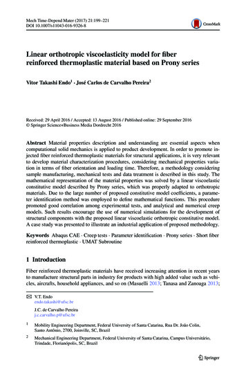
Mech Time-Depend Mater (2017) 21:199–221DOI 10.1007/s11043-016-9326-8Linear orthotropic viscoelasticity model for fiberreinforced thermoplastic material based on Prony seriesVitor Takashi Endo1 · José Carlos de Carvalho Pereira2Received: 29 April 2016 / Accepted: 13 August 2016 / Published online: 29 September 2016 Springer Science Business Media Dordrecht 2016Abstract Material properties description and understanding are essential aspects whencomputational solid mechanics is applied to product development. In order to promote injected fiber reinforced thermoplastic materials for structural applications, it is very relevantto develop material characterization procedures, considering mechanical properties variation in terms of fiber orientation and loading time. Therefore, a methodology consideringsample manufacturing, mechanical tests and data treatment is described in this study. Themathematical representation of the material properties was solved by a linear viscoelasticconstitutive model described by Prony series, which was properly adapted to orthotropicmaterials. Due to the large number of proposed constitutive model coefficients, a parameter identification method was employed to define mathematical functions. This procedurepromoted good correlation among experimental tests, and analytical and numerical creepmodels. Such results encourage the use of numerical simulations for the development ofstructural components with the proposed linear viscoelastic orthotropic constitutive model.A case study was presented to illustrate an industrial application of proposed methodology.Keywords Abaqus CAE · Creep tests · Parameter identification · Prony series · Short fiberreinforced thermoplastic · UMAT Subroutine1 IntroductionFiber reinforced thermoplastic materials have received increasing attention in recent yearsto manufacture structural parts in industry for products with high added value such as vehicles, aircrafts, household appliances, and so on (Masuelli 2013; Tanasa and Zanoaga 2013;B V.T. Endoendo.takashi@ufsc.brJ.C. de Carvalho Pereiraj.c.carvalho.p@ufsc.br1Mobility Engineering Department, Federal University of Santa Catarina, Rua Dr. João Colin,Santo Antônio, 2700, Joinville, SC, Brazil2Mechanical Engineering Department, Federal University of Santa Catarina, Campus Universitário,Trindade, Florianópolis, SC, Brazil
200Mech Time-Depend Mater (2017) 21:199–221Jeyanthi and Rani 2012; Prabhakaran and Kumar 2012; Mertz 2003). The advantages overtraditional materials include, among others, high strength-to-weight ratio and high stiffnessto-weight ratio. These characteristics are directly related to structural applications, in termsof materials selection. Additionally, components made of short fiber reinforced thermoplastic materials have relatively low processing costs, especially if the injection molding processis used (Li 2015; Yang et al. 2013; Östergren 2013; Vélez-García et al. 2011; Araújo et al.2009; Chang and Yang 2001).According to Banks et al. (2011) and Reese and Govindjee (1998), thermoplastic materials exhibit simultaneously elastic and viscous behavior, which depends on material characteristics and microstructure. Fiber reinforced composite materials show anisotropic properties due to fiber orientation and also viscoelastic behavior due to thermoplastic matrix.In order to prevent failure modes related to viscoelastic behavior in structural parts madeof fiber reinforced thermoplastic materials, an overview of available research was performed.Abadi (2008) showed an implicit finite element method to analyze the thermoforming process of thermoplastic sheets reinforced with unidirectional continuous fibers in which thetransient reversible network theory was used to model anisotropic material behavior. Drozdov et al. (2010) derived constitutive equations using finite thermo-viscoelasticity model todescribe polymer melting; parameters were adjusted using experimental curve fitting.In Despringre et al. (2014), a new micromechanical model was used for high cycle fatiguedamage of short glass fiber reinforced Polyamide-66. Proposed material model considereddamage and nonlinear viscoelasticity matrix.Nguyen et al. (2007) presented constitutive models considering anisotropy and finitedeformation viscoelasticity, in which fiber and polymeric matrix can exhibit distinct timedependent behavior. Nedjar (2007) examined a fully three-dimensional constitutive modelfor anisotropic viscoelasticity, which is suitable for the macroscopic description of fiber reinforced composites that experience finite strains. It was considered that the polymeric matrixand the fibers are treated separately, allowing it to represent as many bundles of fibers asdesired. Nedjar (2011) developed a model for the macroscopic description of unidirectionalfiber reinforced composites. Fiber contribution was considered as time-independent and linearly elastic, while viscoelastic matrix experiences creep only in shear. In Chevali (2009),an analysis of creep as a function of variables like fiber length, fiber volume fraction andmaterial degradation due to moisture absorption and ultraviolet radiation was performed.Papadogiannis et al. (2009) evaluated the creep behavior and the viscoelastic properties atdifferent temperatures for glass fiber and carbon fiber endodontic posts.In the work presented by Suchocki (2013), the framework of QLV—Quasi Linear Viscoelastic theory was used to formulate a new rheological model able to capture the nonlinear viscoelastic behavior of thermoplastics and resins. This model was implemented intothe FE—Finite Element system of commercial software Abaqus. In Puso and Weiss (1998),a theoretical and computational framework was developed to apply finite element method toanisotropic viscoelastic soft tissues. A discrete spectrum approximation was developed forQLV relaxation function.Ghazisaeidi (2006) studied the effects of anisotropic material properties of the short glassfiber reinforced thermoplastics on acoustic behavior. Numerical tools were employed toinvestigate steady dynamic responses of the plastic model under a harmonic excitation. Fiberorientation was obtained using injection molding simulation.As noted, studies related to material characterization and constitutive models are requiredto understand viscoelastic behavior of composite parts. These developments, combined witha finite element code, allow a significant improvement of product development process.Due to the lack of a proper model for linear orthotropic viscoelastic materials in currentcommercial finite element packages, the aim of this paper is to implement this constitutive
Mech Time-Depend Mater (2017) 21:199–221201Fig. 1 Fiber orientationmodel as a subroutine and identify its Prony series parameters by fitting numerical andexperimental creep test data. Considering this numerical tool improvement, it is possible tostudy particular failure modes related to viscoelastic behavior in composite parts.2 Materials and methodsThis section describes theory and methodology considered to support research regardingexperimental procedures, data treatment, constitutive model and user subroutine.2.1 Linear orthotropic viscoelasticityIt is well established that mechanical properties of fiber reinforced plastics depend on material orientation. Mechanics of composite materials usually describe longitudinal and transverse directions related to fiber, which are described in Fig. 1.Orthotropic models consider different material behavior for each orthogonally relateddirection. As a consequence, more parameters are needed to fully describe material behaviorwhen compared to isotropic materials. The stiffness matrix of orthotropic materials showingelastic constants is presented in Eq. (1), where the term is defined in Eq. (2): 1 ν23 ν32 ν21 ν31 ν23 ν31 ν21 ν32 0 0 0 EE EE EE 232323σ1 ε1 31 ν13 ν32 ν31 ν12 ν12E νE13 ν32 1 ν 0 0 0 σ2 ε2 E3 E1 E3 E1 3 1 ν ν ν ν ν ν 1 ν ν ε3 σ31312 232313 2112 21000 E1 E2 E1 E2 E1 E2 γ12 ,τ12 00000G12 τ13 γ13 00000G13τ23γ230000 0 G23 1 ν12 ν21 ν23 ν32 ν31 ν13 2ν12 ν23 ν31. E1 E2 E3(1)(2)It should be noted that the Voigt notation is used through the text due to the symmetrictensors; thus, second-order tensors are presented as column matrices with independent components.Materials, in general, can exhibit both instantaneous and time-dependent response. Asa reference for this representation, classic viscoelasticity models proposed by Kelvin andMaxwell describe a spring and a dashpot for instantaneous and time-dependent properties,respectively.
202Mech Time-Depend Mater (2017) 21:199–221Fig. 2 Representation ofgeneralized Maxwell modelViscoelasticity behavior is typically observed as two typical phenomena: creep, whichdescribes a increase in strain due to a constant stress state, and stress relaxation, representinga decrease in stress when structure is subjected to a constant strain (Christensen 2003).Linear viscoelasticity hypothesis assumes that strain increment is linearly proportional tostress, acting as a linear scale factor for creep behavior. This assumption is usually considered valid for small stress levels. Higher stress states or temperatures can induce nonlinearviscoelasticity or even viscoplastic material behavior.2.2 Constitutive model based on Prony seriesGeneralized Maxwell model defines a material representation as a parallel combination of nMaxwell’s spring–dashpot association, as shown in Fig. 2. The mathematical representationof such idealization is a summation of exponential terms defined as Prony series, as shownin Eq. (3). It should be noted that n also corresponds to the number of summation terms ofProny series, as stated by Park (2001) and Tschoegl (1989).n t(3)αi e βii 1whereαi is the first Prony term, andβi is the second Prony term.Commercial FE softwares currently employ Prony series to define time dependency ofstress–strain relation in terms of volumetrical and deviatorical stiffness, as written in Eq. (4).It is important to highlight that only isotropic behavior is typically available in FE programsfor viscoelasticity models, as also stated by Pettermann and Hüsing (2012). tσ (t) 0 dεv K t t dt dt whereK is the volumetric stiffness,G is the deviatoric stiffness,t is the current time,t is the previous time,εv is the volumetric strain, andεd is the deviatoric strain. t0 dεd 2G t t dtdt (4)
Mech Time-Depend Mater (2017) 21:199–221203Based on this representation, volumetrical and deviatorical stiffness are time-dependentfunctions and are typically represented as Prony series, according to Eqs. (5) and (6), respectively: K(t) nK KKzero α i 1 G(t) tKαiK e βi GGzero α nG ,(5).(6) tβGαjG e jj 1The terms Kzero and Gzero represent instantaneous material stiffness and are usually obtained from tensile tests. As the variable t approaches zero, Prony series indicates that material stiffness is dictated only by these instantaneous values. Moreover, α terms are obtainedfrom Eq. (7), as long as Eq. (8) is satisfied. Each αi term is related to the loss of stiffness atthe time indicated by βi . Thus, α represents residual stiffness when time tends to infinity:α 1 n (7)αi ,i 1n αi 1.(8)i 1For the purpose of this work, each elastic term of constitutive model is then formulatedto consider a function of time t using Prony series. It is shown in Eq. (9) as a function ofelastic modulus for longitudinal fiber direction along time t , E1 (t) nE1E1,zero α E1 t E1Eαi 1 e βi(9).i 1Elastic modulus in the transverse direction and shear modulus in the transverse plane,written in terms of Prony series, are presented in Eqs. (10) and (11), respectively: E2 (t) E2E2,zero α n tE2Eαi 2 e βi nG12G12G12,zero α (10),i 1 G12 (t) E2 tG12Gαi 12 e βi .(11)i 1Considering that strain values vary along time, i.e., εx (t) and εy (t), it is also expectedthat Poisson’s ratio becomes a function of time, as represented in Eq. (12):νxy (t) εy (t).εx (t)(12)Therefore, Poisson’s ratio is also written in terms of Prony series, according to Eqs. (13)and (14). It should be noted that we use the inverse function due to the ascending shape of
204Mech Time-Depend Mater (2017) 21:199–221Prony series curves: nν12 t 1ν12 β ν12ν12ν12 (t) ν12,zero α αi e i,(13)i 1 nν21 t 1ν21 β ν21ν21. ν21,zero α αi e iν21 (t)(14)i 1Regarding unidirectional fiber composites, it is possible to simplify orthotropic stiffnessmatrix presented in Eq. (1) as a transversely isotropic material. This assumption considersthat directions 2 and 3 of Fig. 1 show the same properties related to transverse fiber orientation. Therefore, elastic parameters as a function of time, indicated in Eqs. (9), (10), (11),(13), and (14), are finally incorporated into the compliance matrix. According to Klasztorny(2008), obtained Eq. (15) can be considered as the coupled standard equation of monotropicviscoelasticity, written using Voigt notation, namely 1E1 (t) ν12 (t) ε1 (t) E (t) 1 ν12 (t) ε2 (t) E (t)ε3 (t)1 (t)γ 12 0 γ13 (t) 0γ23 (t)0 ν21 (t) ν21 (t)E2 (t)E2 (t) ν21E2 (t)E2 (t) ν21E2 (t)E2 (t)000000000000000100G12 (t)001G12 (t)002(1 ν2 )E2 (t) σ1 (t) σ2 (t) σ3 (t) τ12 (t) . τ13 (t) τ23 (t) (15)2.3 Experimental proceduresMaterial characterization procedures were conducted to identify mechanical properties ofpolybutylene terephthalate (PBT) with 20 % content of glass fiber (GF) reinforcement.Samples for tensile tests are usually obtained from a mold cavity with dimensions indicated by standards. Arjmand et al. (2011) shows schematics of a dog-bone sample obtaineddirectly from injection molding. This procedure becomes limited to isotropic materials, asonly one direction can be evaluated. Therefore, it is not suitable for characterization of fiberreinforced materials.Based on this drawback, an injected plate is proposed to provide samples with differentfiber orientation. It is noteworthy that this injected plate was developed previously and itsintent was to get uniform region in terms of fiber orientation. Rios (2012) performed aninjection molding simulation and indicated that the square region of plate tends to present auniform distribution.Assuming that main region of plate presents uniform fiber orientation, samples werefinally cut accordingly to 0 , 90 and 45 , as shown in Fig. 3. Dimensions were consistentwith ANSI/ASTM D638 and ANSI/ASTM D2990 standards.The waterjet cutting technique was employed to obtain samples in order to prevent polymer degradation during this process. It should be pointed out that degradation was observedin previous attempts using laser cutting. The fiber orientation angle of samples θ , defininglocal (1, 2, 3) and global (x, y, z) coordinate system, is illustrated in Fig. 4.In order to capture longitudinal and transverse strains in time, strain gauges were attached on a sample and a dummy, as shown in Fig. 5. It is important to emphasize that a
Mech Time-Depend Mater (2017) 21:199–221205Fig. 3 Injected plateFig. 4 Fiber orientation angleFig. 5 Strain gauge and a dummyTable 1 Load of creep test foreach sample orientationOrientationLoad (N)Area (mm2 )Stress (MPa)0 468.1538.0612.3090 467.1739.2811.8945 472.0238.8812.14Wheatstone full-bridge configuration was applied in order to prevent eventual thermally related strain measures, as indicated by Rosa (2004) and Malerba et al. (2008). We also wishto highlight the fact that the fiber orientation of the dummy is consistent with the sample.Strain measurements were then stored using data acquisition system HBM Spider 8.Samples were subjected to tensile tests with prescribed displacement ratio of 5 mm/min,as indicated by standards. The duration of each experiment was less than 35 s. Finally,a maximum stress state of 10 MPa was considered as a stopping criterion.Additionally, creep tests were conducted to study viscoelastic behavior. In this experiment, a constant stress state is applied and strain is measured in time. Samples were loadedaccording to Table 1 during approximately 3.5 weeks at a temperature of 23.5 C. A smallvalue of stress state, when compared to yield stress, is intended to preserve linear viscolasticity assumptions.
206Mech Time-Depend Mater (2017) 21:199–2212.4 Data treatmentExperimental data of strain values at various times are converted to time-dependent elasticparameters. Elastic moduli (Eqs. (16) and (17)) and Poisson’s ratios (Eqs. (18) and (19))are obtained from strain values of samples with 0 and 90 fiber orientation, while shearmodulus is identified from results of sample with 45 fiber orientation:σx,0 ,εx,0 (t)σx,90 E2 (t) ,εx,90 (t)E1 (t) (16)(17)ν12 (t) εy,0 (t),εx,0 (t)(18)ν21 (t) εy,90 (t).εx,90 (t)(19)Shear modulus G12 (t) can be written in terms of longitudinal or transverse strain, asdescribed in Eqs. (20) and (21), respectively. As strain values in both longitudinal and transverse directions were collected for the 45 sample, final shear modulus is obtained by takingthe average of both measures, as indicated in Eq. (22):G12,εx (t) G12,εy (t) G12 (t) cos2 (θ ) sin2 (θ )(εx,45 (t)σx,45 cos4 (θ)E1 (t) sin4 (θ)E2 (t) 2ν12 (t) cos2 (θ) sin2 (θ))E1 (t)cos2 (θ ) sin2 (θ )(εy,45 (t)σx,45 cos2 (θ) sin2 (θ)E1 (t) cos2 (θ) sin2 (θ)E2 (t)G12,εx (t) G12,εy (t).2 (20),2ν12 (t) cos4 (θ) sin4 (θ))E2 (t),(21)(22)The value of Poisson ratio of polymer matrix ν2 0.44 was considered constant in time,and it was obtained from manufacturer’s material data sheet. This information is necessaryto define G23 (t), as given in Eq. (23):G23 (t) E2 (t).2(1 ν2 )(23)2.5 Parameter identificationIn order to introduce such material models in a structural analysis, it is important to identifymechanical properties in both longitudinal and transverse directions by performing testsand data treatment. However, the proposed model shows a large number of parameters todescribe viscoelastic behavior in different directions.In this regard, material characterization is aided by numerical models and proper optimization techniques. This so-called parameter identification method consists in findingthe material coefficients by minimizing the difference between experimental and numericalcurves of the same experiment. This procedure is specially useful to characterize nonlinearmaterials, as studied by Khalfallah et al. (2015) and Vaz et al. (2015).
Mech Time-Depend Mater (2017) 21:199–221207Table 2 FE programs used in this workAnsysAbaqusMoldflowParameter identificationStructural analysis with UMATInjection moldingTable 3 Initial values of βiβ1β2β3β4β5β6β72 1002 1012 1022 1032 1042 1052 106For the purpose of this work, a parameter identification tool already implemented inAnsys was employed. Even though it is initially intended for a linear isotropic viscoelastic model, the curve fit algorithm could also be used to find Prony terms of the proposedorthotropic model. As different FE programs were used in the research, Table 2 explainswhich Computer Aided Engineering (CAE) program was utilized for each task.A very useful documentation to describe this Ansys feature was written by Imaoka(2008), which recommends to stipulate initial values for βi , depending on magnitude order of time of creep test. Initial values for these Prony terms, presented in Table 3, allowedconvergence in the optimization process with residual values as low as 1 10 5 .2.6 UMAT—user material subroutineCommercial FE softwares, like Abaqus, allow users and researchers to create their ownmaterial model by writing a Fortran code with a proper stress–strain relation that definesa constitutive model. User material subroutines are extensively used to evaluate differentmaterial behavior from those already implemented in Abaqus.During the iterative trial solution, this external subroutine updates stress state based onstrain values, and force equilibrium is checked as described by Wang et al. (2012).Luo and Lee (2008) evaluated damage of Carbon-Epoxy structures using UMAT. Kimet al. (2013) developed a constitutive model to represent viscoplastic damage of austeniticstainless steel. Both Abaqus subroutine studies showed good agreement between experimental and numerical data, indicating the adequacy of material model and user subroutineimplementation procedures.Implementation of constitutive model allows the evaluation of distinct failure modes ofmaterials, improving numerical simulation capabilities to solve engineering problems. Inthis context, linear orthotropic viscoelastic model can be applied to evaluate short fiber reinforced composites, manufactured by injection molding process. This model can predictnodal displacement along time of a structure when it is subjected to a constant load.It is particularly noteworthy that time t , which is a variable of constitutive model, wasrepresented by the time step value of FE program. Furthermore, material orientation wasapplied using graphical interface of Abaqus.The success of subroutine implementation can be checked by running a numerical creeptest with same parameters as the analytic model. Outputs like strain variation in time in bothlongitudinal and transverse direction are compared. This verification is very important dueto the inherent complexity of programming process and its data transfer to finite elementsolver.Finally, once the subroutine is properly implemented, it is possible to apply such a material model to an arbitrary geometry, making use of all FE benefits in terms of the CAE toolin a product development context.
208Mech Time-Depend Mater (2017) 21:199–221Fig. 6 Tensile test: elasticmoduli E1 and E23 ResultsIn this section, expected results are related to experimental procedures of tensile and creeptests, optimization results of parameter identification method, and finally numerical resultsof subroutine implementation.3.1 Tensile testMaterial stiffness is characterized using averaged stress vs strain curves from tensile tests, asshown in Fig. 6. As a consequence of fiber orientation, it was found that 0 fiber orientationsamples are stiffer when compared to those with 90 fiber orientation.Poisson’s ratio is defined by the negative ratio of transverse to longitudinal strain. As seenin Fig. 7, ν12 and ν21 are observed as the slopes of a line, considering samples with 0 and 90 of fiber orientation, respectively. Based on that experiment, it was found that ν21 0.2948;however, in order to ensure the symmetry of compliance matrix, ν21 was obtained usingEq. (24). Either way, that symmetry is numerically imposed during the solution for properrepresentation of orthotropy model:ν21 E2 ν12.E1(24)Note that shear stiffness is identified with 45 fiber orientation samples, as also mentioned by Yokoyama and Nakai (2007). As it can be seen in Eqs. (25) and (26), shear stressand shear strain can be obtained from experimental data. This procedure is important because, as noted earlier, experimental data are in the global coordinate system (x, y, z):σx,45 ,2(25)γ12 εx,45 εy,45 .(26)τ12 Finally, the definition of shear modulus is shown in Eq. (27),G12 τ12.γ12(27)
Mech Time-Depend Mater (2017) 21:199–221209Fig. 7 Tensile test: Poisson’sratios ν12 and ν21Fig. 8 Tensile test: shearmodulus G12As shown in Fig. 8, shear modulus G12 is identified as the slope of the line relating shearstress and engineering shear strain.As presented previously by Sonnenhohl (2012), the yield stress of Ticona Celanex 3226was determined in the longitudinal and transverse directions as σyield,1 and σyield,2 , respectively. Finally, these so-called instantaneous properties obtained from tensile test are thensummarized in Table 4.3.2 Creep testThe results of creep tests are presented in terms of strain values varying in time. The resultsin longitudinal and transverse direction are presented in Figs. 9 and 10, respectively.
210Mech Time-Depend Mater (2017) 21:199–221Table 4 Elastic properties obtained from tensile testE1 (MPa)E2 (MPa)G12 (MPa)ν12ν21σyield,1 (MPa)σyield,2 (MPa)7178.45976.01874.60.38360.319352.3641.54Fig. 9 Creep test: longitudinalstrain3.3 Parameter identificationExperimental strain data were converted to time-dependent elastic parameters as proposedearlier. Using the parameter identification methodology, the unknowns of orthotropic viscoelastic constitutive model can be properly specified. The Prony series parameters of elastic modulus, shear modulus and Poisson’s ratio are finally presented in Tables 5, 6 and 7,respectively. It should be noted that a large number of coefficients are needed for each material property, as a consequence of a constitutive model using 7 Prony terms. Previous testsusing fewer Prony terms indicated poor material representation; this finding is corroboratedby Imaoka (2008), who described a recommendation regarding the number of Prony termsas dependent on the magnitude order of the total time of creep test experiment.In order to verify obtained parameters, curves of material properties varying in time areplotted comparing experimental and analytical data. Elastic modulus, shear modulus andPoisson’s ratio are illustrated in Figs. 11, 12 and 13, respectively.Good agreement between experimental and analytical curves was found, highlightingthe fact that analytical ones employed Prony parameters obtained earlier. As can be seenin Table 8, consistent values were found for most elastic parameters obtained from tensile
Mech Time-Depend Mater (2017) 21:199–221211Fig. 10 Creep test: transversestrainTable 5 Polybutyleneterephthalate (20 % content ofglass fiber): elastic modulusiE1 (t)E1,zero7230E11234567E2 (t)Eα 1E2,zeroα 20.6182159200.57300E1E2EE2αiβiαiβi1.4 10 86.068 1001.7 10 81.611 1020.0810564.063 1010.1060204.171 1010.0218554.829 1020.0277969.609 1020.0622663.996 1030.0618105.299 1030.0315724.066 1040.0332714.285 1040.0899001.785 1050.0940281.963 1050.0951361.419 1060.1040701.536 106and creep tests. Based on the creep test, it was found that ν21 0.2801; however, in orderto ensure symmetry of the compliance matrix, ν21 was obtained using Eq. (24). Therefore,instantaneous Poisson’s ratio should be modified to ν23,zero 3.14.3.4 Numerical simulationAs the constitutive model is implemented in a commercial FE program, a numerical creeptest was conducted employing identified material parameters. Therefore, a solid mesh model
212Table 6 Polybutyleneterephthalate (20 % content ofglass fiber): shear modulusMech Time-Depend Mater (2017) 21:199–221iG12 (t)G12,zero2160G12GG23,zeroα .160 1004.8 10 85.312 1030.1542001.500 1010.1060204.171 1010.0476415.615 1020.0277969.609 1020.0788854.142 1030.0618105.299 1030.0424974.305 1040.0332714.285 1040.1060501.840 1050.0940281.963 10570.1053901.317 1060.1040701.536 106i(ν12 (t)) 1123456Table 7 Polybutyleneterephthalate (20 % content ofglass fiber): Poisson’s ratiosG23 (t)Gα 12(ν21 (t)) 1ννν12,zeroα 12ν23,zeroα 232.570.901943.570.95785νννναi 12βi 12αi 23βi 2310.0081007.628 1005.4 10 30.917 10022.2 10 8345671.858 1013.1 10 1031.995 1010.0017372.081 1024.3 10 130.0192951.982 1030.0075052.000 1030.0080472.000 1040.0034912.000 1040.0372332.000 1050.0257732.000 1050.0236682.000 1060.0000002.000 106Table 8 Properties obtainedfrom tensile and creep testTensile testCreep test2.000 102 0.72%E1 (MPa)71787230E2 (MPa)597659200.94%G12 (MPa)18752160 15.20%ν120.38360.3891 1.43%ν210.31930.31850.25%representing the test sample subjected to constant stress state according to Table 1 was evaluated in time.Strain values in both longitudinal and transverse directions were recorded from simulation and presented to be compared to analytical ones. The creep test results of samples withfiber orientation angle of 0 , 90 and 45 are shown in Figs. 14, 15 and 16, respectively.These comparative results indicated that the subroutine implementation was performed successfully.
Mech Time-Depend Mater (2017) 21:199–221213Fig. 11 Parameter identificationresults: elastic modulusFig. 12 Parameter identificationresults: shear modulus3.5 Industrial application: injection molding and structural simulationConsidering that the material subroutine was properly implemented in a commercial FEprogram, it is possible to apply such a constitutive model to perform structural analysis of aproduct. In other words, this methodology allows engineers to check failure modes relatedto viscoelastic behavior. For instance, for some applications it might be interesting to predictand evaluate displacement over time in a fiber reinforced product subjected to constant load.It is important to highlight the fact that stress state is compatible with linear viscoelasticbehavior, otherwise simulation would provide misleading results.A case study is presented in this section to exemplify an industrial application of themethodology presented in this paper. The fiber orientation was obtained via an injectionmolding simulation, and this information was imported into a structural finite element program using solid mesh. As mechanical properties are functions of fiber orientation, it isimportant to perform a manufacturing process simulation and then import such data to struc-
214Mech Time-Depend Mater (2017) 21:199–221Fig. 13 Parameter identificationresults: Poisson’s ratioFig. 14 Strain variation in time:sample with θ 0 tural analysis. This is an analogous procedure to that when considering residual stresses dueto the forming process in a sheet metal part.Fiber orientation is a result of the filling stage of the injection process which can be evaluated using numerical tools. Moldflow simulation indicates a prediction of fiber orientationdue to the filling stage of injection molding,
a theoretical and computational framework was developed to apply finite element method to anisotropic viscoelastic soft tissues. A discrete spectrum approximation was developed for QLV relaxation function. Ghazisaeidi (2006) studied the effects of anisotropic material properties of the short glass fiber reinforced thermoplastics on acoustic .