Transcription
Plotting Haplotype Networks with pegasEmmanuel ParadisFebruary 10, 2021Contents1Introduction12The Function plot.haploNet2.1 Node Layout . . . . . . . . . . . . . . . . . . . . . . . . . . . . . . . . . . . .2.2 Options . . . . . . . . . . . . . . . . . . . . . . . . . . . . . . . . . . . . . . .1253New3.13.23.33.41Features in pegas 1.0Improved “Replotting” . . . .Haplotype Symbol Shapes . .The Function mutations . . .Getting and Setting Options .1010111315IntroductionHaplotype networks are powerful tools to explore the relationships among individuals characterised with genotypic or sequence data [3, 5]. pegas has had tools to infer and plothaplotype networks since its first version (0.1, released in May 2009). These tools have improved over the years and are appreciated in the community working on population geneticsand genomics (see John Bhorne’s blog1 ).This document covers some aspects of drawing haplotype networks with pegas with anemphasis on recent improvements. Not all details and options are covered here: see therespective help pages (?plot.haploNet and ?mutations) for full details. The functionplotNetMDS, which offers an alternative approach to plot networks, is not considered in thisdocument.2The Function plot.haploNetThe current version of pegas includes five methods to reconstruct haplotype networks aslisted in the table below.MethodAcronymInput dataFunctionRef.Parsimony networkMinimum spanning treeMinimum spanning networkRandomized minimum spanning treeMedian-joining etmstmsnrmstmjn[6][4][1][5][1]1 in-r/1
All these functions output an object of class "haploNet" so that they are plotted with thesame plot method.2.1Node LayoutThe coordinates of the nodes (or vertices) representing the haplotypes are computed intwo steps: first, an equal-angle algorithm borrowed from Felsenstein [2] is used, second thespacing between nodes is optimised. The second step is ignored if the option fast TRUEis used when calling plot.In the first step, the haplotype with the largest number of links is placed at the centreof the plot (i.e., its coordinates are x y 0), then the haplotypes connected to this firsthaplotype are arranged around it and given equal angles. This is then applied recursivelyuntil all haplotypes are plotted. To perform this layout, an initial “backbone” network basedon an MST is used, so there are no reticulations and the equal-angle algorithm makes surethat there are no segment-crossings. In practice, it is likely that this backbone MST isarbitrary with respect to the rest of the network. The other segments are then drawn on“top” of this MST.In the second step, a “global energy” is calculated based on the spaces between the nodesof the network (closer nodes imply higher energies). The nodes are then moved repeatedly,while keeping the initial structure of the backbone MST, until the global energy is notimproved.We illustrate the procedure with the ‘woodmouse’ data, a set of sequences of cytochromeb from fifteen woodmice (Apodemus sylvaticus): library(pegas) # loads also ape data(woodmouse)In order, to simulate some population genetic data, we sample, with replacement, eightysequences, and create two grouping, hierarchical variables: region with two levels eachcontaining forty haplotypes, and pop with four levels each containing twenty haplotypes: set.seed(10)x - woodmouse[sample.int(nrow(woodmouse), 80, TRUE), ]region - rep(c("regA", "regB"), each 40)pop - rep(paste0("pop", 1:4), each 20)table(region, pop)popregion pop1 pop2 pop3 pop4regA202000regB002020We extract the haplotypes before reconstructing the RMST after computing the pairwiseHamming distances: h - haplotype(x) hHaplotypes extracted from: xNumber of haplotypes: 15Sequence length: 965Haplotype labels and frequencies:IIIIIIIVVVIVII VIII2IXXXIXII XIIIXIVXV
5693774637763 d - dist.dna(h, "N") nt - rmst(d, quiet TRUE) ntHaplotype network with:15 haplotypes22 linkslink lengths between 2 and 14 stepsUse print.default() to display all elements.We now plot the network with the default arguments: plot(nt)IVIIIVIIIVIIIXIIIXXIVVIIXXIIIIVXIXVWe compare the layout after setting fast TRUE:352
plot(nt, fast TRUE)IVVIIIIXIVVIIVIXIIIXIIIIXXIIIIVXIXVBy default, not all links are drawn. This is controlled by the option threshold which takestwo values to set the lower and upper bounds of the number of mutations for a link to bedrawn: plot(nt, threshold c(1, 14))4
IVIIIVIIIVIIIXIIIXXIVVIIXXIIIIVXIXVThe visual aspect of the links is arbitrary: the links of the backbone MST are shown withcontinuous segments, while “alternative” links are shown with dashed segments.2.2Optionsplot.haploNet has a relatively large number of options: args(pegas:::plot.haploNet)function (x, size 1, col, bg, col.link, lwd, lty, shape "circles",pie NULL, labels, font, cex, scale.ratio, asp 1, legend FALSE,fast FALSE, show.mutation, threshold c(1, 2), xy NULL,.)NULLLike for most plot methods, the first argument (x) is the object to be plotted. Until pegas0.14, all but the first arguments were defined with default values. In recent versions, asshown above, only size and shape are defined; the other options, if not modified in thecall to plot, are taken from a set of parameters which can be modified as explained inSection 3.4.The motivation for this is, in most practical applications of this function, the user will5
want to modify size and shape with their own data such as the haplotype frequencies orelse, and they might be changed repeatedly, for instance with different data subsets. On theother hand, the other options are more likely to be used to change the visual aspect of thegraph so it could be more useful to change them once during a session as explained below.The size of the haplotype symbols can be used to display haplotype frequencies. Thefunction summary can extract these frequencies from the "haplotype" object: (sz - summary(h))I5II6III9IV3V7VI7VII VIII46IX3X7XI7XII XIII63XIV5XV2It is likely that these values are not ordered in the same way than haplotypes are orderedin the network: (nt.labs - attr(nt, "labels"))[1] "VII"[11] "II""XV""V""I""XII""XIII" "III""IV""XI""IX""VI""X"It is simple to reorder the frequencies before using them into plot: sz - sz[nt.labs] plot(nt, size sz)6"VIII" "XIV"
IIVVIIVIIIXIVIIIVIXIIIXIXXIIIIVXIXVA similar mechanism can be used to show variables such region or pop. The functionhaploFreq is useful here because it computes the frequencies of haplotypes for each regionor population: (R - haploFreq(x, fac region, haplo h))regA II15XIII21XIV14XV027
(P - haploFreq(x, fac pop, haplo h))IIIIIIIVVVIVIIVIIIIXXXIXIIXIIIXIVXVpop1 pop2 pop3 23020101130011Like with size, we have to reorder these matrices so that their rows are in the same orderthan in the network: R - R[nt.labs, ] P - P[nt.labs, ]We may now plot the network with either information on haplotype frequencies by justchanging the argument pie: plot(nt, size sz, pie R, legend c(-25, 30))8
I25 9regAregBIVVIIVIIIXIVIIIVIXIIIXIXXIIIIVXIXV plot(nt, size sz, pie P, legend c(-25, 30))9
I25 XVNew Features in pegas 1.0This section details some of the improvements made to haplotype network drawing afterpegas 0.14.3.1Improved “Replotting”The graphical display of networks is a notoriously difficult problem, especially when there isan undefined number of links (or edges). The occurrence of reticulations makes line crossingsalmost inevitable. The packages igraph and network have algorithms to optimise the layoutsof nodes and edges when plotting such networks.The function replot (introduced in pegas 0.7, March 2015) lets the user modify the layoutof nodes interactively by clicking on the graphical window where a network has been plottedbeforehand. replot—which, of course, cannot be used in this non-interactive vignette—hasbeen improved substantially: The explanations printed when the function is called are more detailed and the nodeto be moved is visually identified after clicking.10
The final coordinates, for instance saved with xy - replot(), can be used directlyinto plot(nt, xy xy). This makes possible to input coordinates calculated withanother software. In previous versions, the plot tended to “drift” when increasing the number of nodemoves. This has been fixed, and the network is correctly displayed whatever thenumber of moves done.3.2Haplotype Symbol ShapesHaplotypes can be represented with three different shapes: circles, squares, or diamonds.The argument shape of plot.haploNet is used in the same way than size as explainedabove (including the evental need to reorder the values). Some details are given belowabout how these symbols are scaled.There are two ways to display a quantitative variable using the size of a circle: eitherwith its radius (r) or with the area of the disc defined by the circle. This area is πr2 , so if wewant the area of the symbols to be proportional to size, we should square-root these lastvalues. However, in practice this masks variation if most values in size are not very different(see below). In pegas, the diameters of the circles (2r) are equal to the values given by size.If these are very heterogeneous, they could be transformed with size sqrt(. keepingin mind that the legend will be relative to this new scale.The next figure shows both ways of scaling the size of the circles: the top one is thescaling used in pegas. par(xpd TRUE)size - c(1, 3, 5, 10)x - c(0, 5, 10, 20)plot(0, 0, type "n", xlim c(-2, 30), asp 1, bty "n", ann FALSE)other.args - list(y -5, inches FALSE, add TRUE,bg rgb(1, 1, 0, .3))o - mapply(symbols, x x, circles sqrt(size / pi),MoreArgs other.args)other.args y - 5o - mapply(symbols, x x, circles size / 2,MoreArgs other.args)text(x, -1, paste("size ", size), font 2, col "blue")text(30, -5, expression("circles "*sqrt(size / pi)))text(30, 5, "circles size / 2")11
151005circles size / 2size 10 5size 1 size 3 size 5 15 10circles size π051015202530For squares and diamonds (shape "s" and shape "d", respectively), they are scaledso that their areas are equal to the discs for the same values given to size. The figure belowshows these three symbol shapes superposed for several values of this parameter. Note thata diamond is a square rotated 45 around its center. x - c(0, 6, 13, 25)plot(0, 0, type "n", xlim c(-2, 30), asp 1, bty "n", ann FALSE)other.args y - 0o - mapply(symbols, x x, circles size/2, MoreArgs other.args)other.args col - "black"other.args add - other.args inches - NULLo - mapply(pegas:::square, x x, size size, MoreArgs other.args)o - mapply(pegas:::diamond, x x, size size, MoreArgs other.args)text(x, -7, paste("size ", size), font 2, col "blue")12
151050 5size 3size 5size 10 15 10size 103.351015202530The Function mutationsmutations() is a low-level plotting function which displays information about the mutationsrelated to a particular link of the network. This function can be used interactively. Forinstance, the following is copied from an interactive R session: mutations(nt)Link is missing: select one below1: VII-I2: VII-VIII3: V-XI4: III-VI5: IX-X6: IX-II7: III-IX8: VII-III9: XV-V10: XIII-IX11: IX-V12: IX-XII13
-XIIX-IVI-VIIII-IIIXIV-IVII-XIII-VEnter a link number: 18Coordinates are missing: click where you want to place the annotations:The coordinates x -8.880335, y 16.313 are usedThe values entered interactively can be written in a script to reproduce the figure: plot(nt) mutations(nt, 18, x -8.9, y 16.3, data h)I213: T C409: T CVIIIVIIIVIIIXIIIXXIVVIIXXIIIIVXIXVLike any low-level plotting function, mutations() can be called as many times as needed to14
display similar information on other links. The option style takes the value either "table"(the default) or "sequence". In the second case, the positions of the mutations are drawnon a horizontal segment representing the sequence: plot(nt) mutations(nt, 18, x -8.9, y 16.3, data h) mutations(nt, 18, x 10, y 17, data h, style "s")I213: T C409: T CVIIIVIIIVIIIXIIIXXIVVIIXXIIIIVXIXVThe visual aspect of these annotations is controlled by parameters as explained in the nextsection.3.4Getting and Setting OptionsThe new version of pegas has two ways to change some of the parameters of the plot:either by changing the appropriate option(s) in one of the above functions, or by setting these values with the function setHaploNetOptions, in which case all subsequentplots will be affected.2 The list of the option values currently in use can be printedwith getHaploNetOptions. There is a relatively large number of options that affect either plot.haploNet() or mutations(). Their names are quite explicit so that the user will2 See?par for a similar mechanism with basic R graphical functions.15
find which ones to modify: show.mutation"We see here an example with the command plot(nt, size 2) which is repeated aftera call to setHaploNetOptions: plot(nt, size 2)16
IVIIVIIIIVIIIXIIIXXIVVIIXXIIIIVXIXV setHaploNetOptions(haplotype.inner.color "#CCCC4D", haplotype.outer.color "#CCCC4D", show.mutation 3, labels FALSE) plot(nt, size 2)17
2 2271410367384727 setHaploNetOptions(haplotype.inner.color "blue", haplotype.outer.color "blue", show.mutation 1) par(bg "yellow3") plot(nt, size 2)18
setHaploNetOptions(haplotype.inner.color "navy", haplotype.outer.color "navy") par(bg "lightblue") plot(nt, size 2)19
References[1] H. J. Bandelt, P. Forster, and A. Röhl. Median-joining networks for inferring intraspecificphylogenies. Molecular Biology and Evolution, 16(1):37–48, 1999.[2] J. Felsenstein. Inferring Phylogenies. Sinauer Associates, Sunderland, MA, 2004.[3] D. H. Huson and D. Bryant. Application of phylogenetic networks in evolutionary studies.Molecular Biology and Evolution, 23(2):254–267, 2006.[4] J. B. Kruskal, Jr. On the shortest spanning subtree of a graph and the traveling salesmanproblem. Proceedings of the American Mathematical Society, 7(1):48–50, 1956.[5] E. Paradis. Analysis of haplotype networks: the randomized minimum spanning treemethod. Methods in Ecology and Evolution, 9(5):1308–1317, 2018.[6] A. R. Templeton, K. A. Crandall, and C. F. Sing. A cladistic analysis of phenotypicassociation with haplotypes inferred from restriction endonuclease mapping and DNAsequence data. III. Cladogram estimation. Genetics, 132:619–635, 1992.20
haplotype networks since its rst version (0.1, released in May 2009). These tools have im-proved over the years and are appreciated in the community working on population genetics and genomics (see John Bhorne's blog1). This document covers some aspects of drawing haplotype networks with pegas with an emphasis on recent improvements.