Transcription
Haplotype analysisShaun Purcellspurcell@pngu.mgh.harvard.eduMGH, Boston
OverviewWhat are haplotypes?Recombination and linkage disequilibriumHow do we measure haplotypes?Estimating haplotype phase and frequencyHow can we use haplotypes to map causal variants?Haplotype-based association analysis
What is association?Categorical traitsdisease susceptibility genesContinuous traitsquantitative trait loci, QTL
Linkage disequilibrium mappingGenotyped markers
Linkage disequilibrium mappingGenotyped markersQTL
Linkage disequilibrium mappingGenotyped markersQTLUngenotyped markers
RecombinationHomologous chromosomes in one parentPaternal chromosomeMaternal chromosomeRecombination eventduring meiosisRecombinant gamete transmitted,harboring mutation
Homologous chromosomes in one parentPaternal chromosomeMaternal chromosomeNo recombination eventduring meiosisNonrecombinant gamete transmittednot harboring mutation
Linkage: affected sib pairsPaternal chromosomeMaternal chromosomeFirst affected offspring,no recombinationSecond affected offspring,recombinant gameteIBD sharing from this one parent (0 or 1)10
Mutation occurs on a ‘red’ chromosome
Mutation occurs on a ‘red’ chromosome
Association due to linkage disequilibrium’
HaplotypesAMmaaMamThis individual has aa and Mm genotypesand am and aMhaplotypes
MmAAMaaMamThis individual has Aa and Mm genotypeand AM and am haplotypes
MmAAMaaMamThis individual has Aa and Mm genotypeand AM and am haplotypes but given only genotype data,consistent with Am/aM as well as AM/am
MmAAMAmaaMamThis individual has AA and Mmgenotypesand AM and Amhaplotypes
Haplotype analysis1. Estimate haplotypes from genotypes2. Associate haplotypes with traitHaplotypeAAGGAAGTCGCGAGCTFreq.40%30%25%5%Odds Ratio1.00*2.211.070.92* baseline, fixed to 1.00
Measuring haplotypesExpectation – Maximisation algorithmApplicable in situations where there are morecategories than can be distinguishedi.e. ‘incomplete data problems’Complete data ( Observed data , Missing data )Haplotype data ( Genotype data , Phase data )
Measuring haplotypesGenotypesHaplotypesA/A B/b C/cABC / AbcorABc / AbCPhases
E-M algorithm1. Guess haplotype frequencies2. (E) Use those frequencies to replace ambiguousgenotypes with fractional haplotype counts3. (M) Estimate frequency of each haplotype bycounting4. Repeat (2) and (3) until convergence
Dataset to be phased4 individuals genotyped for 2 diallelic markersID1ID2ID3ID4A/AA/aA/aa/aB/Bb/bB/bb/b
Dataset to be phased4 individuals genotyped for 2 diallelic markersID1ID2ID3ID4A/AA/aA/aa/aB/Bb/bB/bb/bAB / ABAb / abAB / ab ? Ab / aBab / ab
E-stepReplace ambiguous A/a B/b genotype with :AB / ab :Ab / aB :
E-stepPAB 0.25PaB 0.25PAb 0.25Pab 0.25Replace ambiguous A/a B/b genotype with :AB / ab : 2 PAB PabAb / aB : 2 PAb PaB
E-stepPAB 0.25PaB 0.25PAb 0.25Pab 0.25Replace ambiguous A/a B/b genotype with :AB / ab : 2 PAB Pab 2 0.25 0.25 0.125 0.125/(0.125 0.125) 0.50Ab / aB : 2 PAb PaB 2 0.25 0.25 0.125 0.125/(0.125 0.125) 0.50
E-stepIncomplete dataA/AB/BComplete dataAB / ABA/ab/bAb / abA/aB/bAB / abAb / aBa/ab/bab / abCount1.001.000.500.501.00
M-stepIncomplete dataA/AB/BComplete dataAB / ABA/ab/bAb / abA/aB/bAB / abAb / aBa/ab/bab / abCount1.001.000.500.501.00Counting AB haplotype 2 1 1 0.5 2.5
M-stepIncomplete dataA/AB/BComplete dataAB / ABA/ab/bAb / abA/aB/bAB / abAb / aBa/ab/bab / abCounting aB haplotype 1 0.5 0.5Count1.001.000.500.501.00
M-stepIncomplete dataA/AB/BComplete dataAB / ABA/ab/bAb / abA/aB/bAB / abAb / aBa/ab/bab / abCount1.001.000.500.501.00Counting Ab haplotype 1 1 1 0.5 1.5
M-stepIncomplete dataA/AB/BComplete dataAB / ABA/ab/bAb / abA/aB/bAB / abAb / aBa/ab/bab / abCount1.001.000.500.501.00Counting ab haplotype 1 1 1 0.5 2 1 3.5
M-stepHaplotype counts, frequencies from complete 50.18750.43751.0000
back to the E-step .PAB 0.25PaB 0.25PAb 0.25Pab 0.25are now replaced withthe updated estimatesPAB 0.3125PaB 0.0625PAb 0.1875Pab 0.4375
back to the E-step .PAB 0.25PaB 0.25PAb 0.25Pab 0.25are now replaced withthe updated estimatesPAB 0.3125PaB 0.0625PAb 0.1875Pab 0.4375Replace ambiguous A/a B/b genotype with :AB / ab : 2 PAB Pab 2 0.3125 0.4375 0.273 0.273/(0.273 0.023) 0.92Ab / aB : 2 PAb PaB 2 0.1875 0.0625 0.023 0.023/(0.273 0.023) 0.08
back to the M-step Incomplete dataA/AB/BComplete dataAB / ABA/ab/bAb / abA/aB/bAB / abAb / aBa/ab/bab / abCount1.001.000.920.081.00Counting AB haplotype 2 1 1 0.92 2.92
back to the M-step Incomplete dataA/AB/BComplete dataAB / ABA/ab/bAb / abA/aB/bAB / abAb / aBa/ab/bab / abCount1.001.000.920.081.00Counting aB haplotype 1 0.08 0.08
back to the M-step Incomplete dataA/AB/BComplete dataAB / ABA/ab/bAb / abA/aB/bAB / abAb / aBa/ab/bab / abCount1.001.000.920.081.00Counting Ab haplotype 1 1 1 0.08 1.08
back to the M-step Incomplete dataA/AB/BComplete dataAB / ABA/ab/bAb / abA/aB/bAB / abAb / aBa/ab/bab / abCount1.001.000.920.081.00Counting ab haplotype 1 1 1 0.92 2 1 3.92
back to the M-step Haplotype counts, frequencies from complete 0100.1350.4901.0000
and back, again, to the E-step and back, again, to the M-step and back, again, to the E-step and back, again, to the M-step and back, again, to the E-step and back, again, to the M-step
Haplotype frequency estimatesi0i1i2 iNAB0.2500.3150.365 0.375aB0.2500.06250.010 0.000Ab0.2500.18750.135 0.125ab0.2500.4375.0.490 0.500
Posterior probabilitiesGenotypePhaseP(H G)A/AB/BAB / AB1.00A/ab/bAb / ab1.00A/aB/bAB / abAb / aBa/ab/bab / ab 1.001.000.00
Missing genotype dataA/A 0/0 c/cPhaseABc / ABcABc / AbcAbc / Abcconsistent with 3 phasesP(H G)( PABc PABc ) / S( 2 PABc PAbc ) / S( PAbc PAbc ) / Swhere S PABc PABc 2 PABc PAbc PAbc PAbc
Using parental genotypesCan often help to resolve phaseA/a B/b C/c
Using parental genotypesCan often help to resolve phaseA/A B/B C/ca/a b/b c/cA/a B/b C/c
Using parental genotypesCan often help to resolve phaseA/A B/B C/ca/a b/b c/cA/a B/b C/cABC / abc
Using parental genotypesCan often help to resolve phaseA/A B/B C/ca/a b/b c/cA/a B/b C/cABC / abc but not alwaysA/a B/b C/cA/a B/b c/cA/a B/b C/c
A (slightly) less trivial example1111212?2121112?3221112211 / 2124121211?5121112?6112222122 / 1227121122112 / 2128221111211 / 2119121222?10222222222 / 222
haplotype 001234567891011E-M iteration121314151617
1121314151617
Haplotype 0000
ID1111chr1212Hap111122112121P(H 00004110.00004110.99995890.9999589IDchrHapP(H 22221.00000001.0000000
A (slightly) less trivial example1111212112 / 1212121112112 / 2113221112211 / 2124121211121 / 2115121112112 / 2116112222122 / 1227121122112 / 2128221111211 / 2119121222112 / 222 ? 122 / 21210222222222 / 222
But it's not always this easy.For m SNPs there are 2m possible haplotypes2m-1 (2m 1) possible haplotype pairsFor m 10 then1,024 possible haplotypes524, 800 possible haplotype pairs
Linkage equilibriumMmAprqrrapsqsspq
Linkage disequilibriumMmApr Dqr - Draps - Dqs DspqDMAX Min(qs, pr)D’ D /DMAXP(A)P(M)r2 D2 / pqrse.g D P(AM) -
Practical sessions Visualising data and testing for associationin Haploview Detecting haplotpe association using whap Fitting nested model to explore theassociation using whap
Practical 1 : HaploviewFolder F:\pshaun\haplotype\ Pedigree format: data1234.ped Case/control sample (N 200 200) Load data into Haploview Examine LD and block structure Examine single SNP association Examine haplotype-based association
Sample filesdataACGT.ped1 A 1 0 0 12 A 1 0 0 1.1 B 1 0 0 12 B 1 0 0 1data1234.ped.1 A 1 0 0 1.dataACGT.datA diseaseM snp1M snp2M snp3M snp422A AA AC CA CC AC AG GT GC CA C11C CA CC CC CC CA CG GG GA AC A21 12 22 13 32 2dataACGT.map1 snp1 0 11 snp2 0 21 snp3 0 31 snp4 0 4pedstats1 snp50 5-p data1234.ped -d data123
LD, block structureBased on default “Gabriel blocks”
Single SNP association
Block-based haplotype tests
The true modelGeneral population haplotype .200.200.050.05Increases risk for disease
Implied from block AGCTrue modelAAATAACAGCCCCGACCCGCAACTAACCGCSignificantly associated with increased riskSignificantly associated with decreased risk
Manually specifying the 'block'
Results with 5-SNP block
whap Numerous recent methods using GLM approachSchaid et al (02) AJHGZaykin et al (02) Hum HeredSeltman et al (03) Genet EpiQuantitative and qualitative traitsMixture of regressions frameworkBetween/within family modelModel either L(X G) or L(G X)Independent secondary test, 1 dfFlexible specification of nested submodels
Single locus analysis Fulker et al (1999)S1S2S1S2BWS1S2AAAA1110B WB-WAAAa100.50.5B WB-WAAaa1-101B WB-WNote : W S1 – B
Parental genotypes Use parental genotypes togenerate BExamplesAA from AAxAAAa from AAxAaAa from AaxAaW 0W -0.5W -1
Available tests X N( bB wW , δ2 )Basic test HA : b wH0 : b w 0Robust test HA : b, wH0 : b , w 0Test for stratification HA : b, wH0 : b wRobust test (2) HA : b 0, wH0 : b w 0
Analysis of selected samples
Conditioning on trait values Model likelihood of observing genotypeconditional on trait valueLGXL XG LGL XG L GSingletons: G { AA, Aa, aa }Pairs: G { AA/AA, AA/Aa, AA/aa, }With parents: G { AA AAxAA, AA AAxAa, }G { AA/AA AAxAA, AA/AA AAxAa, }
Robust in selected samples Type I error ratesSib pairs10% extreme selectionWithin sibship testL(X G) L(G X)Full sampleNo parents5.45.4Parents5.25.0Selected sampleNo parents26.75.3Parents13.85.0
Extension to haplotype analysis Probabilistic haplotype reconstruction viaE-M algorithmAA BB cc DdABcD / ABcdP(P1) 1.00AA Bb cc DdABcD / Abcd P(P1) 0.85ABcd / AbcD P(P2) 0.15
Weighted likelihood Individual i has G consistent phasesL X G LGGEstimated via E-M algorithm
Quantitative & qualitative traits Quantitative traitsL X GL XGg ip ,s 211 e Qualitative traits B [phase x haplotype] matrix of scoresβ [haplotype x 1] vector of regression coefficientsc is a constant gip
Example B matrixIndividual i Genotypes:1/1 1/1 1/1Haplotypes:111 / 111 P() 1.0111g 212101220B matrix222011202210b1 2b1L(G g) 1.0b2b3b4b5Vector ofb6regression coefficients
Example B matrixIndividual j Genotypes:1/1 1/2 1/2Haplotypes:112 / 121 P() 0.8111 / 122 P() 0.2111g 011211012201222001121022100b1 b2 b5 L(G g) 0.8b2b1 b30.2b3b4b5b6
Testing nested hypotheses Test effect of a locus conditional on haplotypebackground. e.g. drop the 3rd locus111g 011211012201222001121022100c1c2c2c3c1c3 c2 c1c1 c2b1 b5b2 b3b4 b6
Parental genotypes Phase parental genotypes via E-MParental phase P(PP,M) P(PP) P(PM) For each PP,M enumerate offspring phases,PC consistent with GCCalculate P(PC PP,M)Can allow for recombination Weighted likelihood over all PP,M and PC
Between/within partitioningB matrix depends on parental phase W G-B To calculate B for a specific PP,Maverage all possible PC given PP,M i.e. whether or not consistent with GC
Between/within partitioningIndividual kGenotypes: 1/11/2Parental Genotypes:1/11/1Parental Haplotypes:11 / 1111 / 11Haplotypes parents 11/11 X11/22:Haplotypes parents 11/11 X12/12:XXXConsistent withoffspring genotypes11 / 121/21/211 / 2212 / 12All possible11 / 1111 / 2211 / 12
Between/within partitioning1/1 1/2 1/2 1/1 0/0 2/2Seven haplotypes 1%212 111 211 112222 122 1211/1 2/2 2/2212 111 211 112 222 122 121212 111 211 112 222 122 121122\111 X 112\122122\111 X 122\112122\111 X 122\122111\122 X 112\122111\122 X 122\112111\122 X 122\122 .0000.0000.0000.0000.0000.0000.000Offspring matrix[ 0.000 0.000 0.000 0.000 0.000 2.000 0.000 00.0000.0000.0000.000]]]]]]]]
Two main types of test Haplotype-specific testsH tests each with 1 dfcompare each haplotype versus all otherscorrection for multiple tests not built-in bus testsingle test with H-1 dfcompare each haplotype against an(arbitrary) reference haplotypebuilt-in correction for multiple tests
Secondary analysis H haplotypes will have H-1 coefficientsReduces power of test – high degrees offreedom More similar haplotypes should have moresimilar effects
Cladogram-collapsingJ 011000000D 010000000H 000100000A 000000000 K 110000000I 000010000B 100000000G 100001100C 100001000E 100001001 F 100001010 After Seltman et al (
Cladogram-collapsingJ 011000000D 010000000H 000100000A 000000000 K 110000000I 000010000B 100000000G 100001100C 100001000E 100001001 F 100001010 After Seltman et al (
Cladogram-collapsingJ 011000000D 010000000H 000100000A 000000000 K 110000000I 000010000B 100000000G 100001100C 100001000E 100001001 F 100001010 After Seltman et al (
Cladogram-collapsingJ 011000000D 010000000H 000100000A 000000000 K 110000000I 000010000B 100000000G 100001100C 100001000E 100001001 F 100001010
Cladogram-collapsingJ 011000000D 010000000H 000100000A 000000000 K 110000000I 000010000B 100000000G 100001100C 100001000E 100001001 F 100001010
Secondary analysis111111-0-112111 111221-0-1111-0-122211 121222-0-1112-X-12221222-X-12222222-X-22
Secondary ated coefficients0.000-0.0920.102-0.2340.6340.3320.865
Secondary analysis Haplotype similarityGlobal and local identity1111112212 1111112212 11111122121111121222 1111121222 1111121222Local 1 (0.5) Local 8 (0.1)Global (0.7) Haplotype effect similaritySquared difference in MLE regressioncoefficients( b1 – b2 )2 ( 0.405 - 0.620 )2 0.462
Sliding window analysisM1M2TaTaM3TbM4TcM5TdM6TeM7TfM8Tg(Ta Tb)/2 (Tb Tc)/2 (Tc Td)/2 (Td Te)/2 (Te Tf)/2 (Tf Tg)/2Tg
For full details: http://www.broad.mit.edu/ shauFile formats QTDT/Merlin input formatdata.datdata.ped1 1 0 0 1 -91 2 A A T quant11 2 0 0 2 -9 2 2 C C M rs0000011 3 1 2 1 -0.23 1 2 A C M rs000002 data.map14 rs00000114 rs0000020 1232320 123887Example command lineswhap --file data --alt 5,6,7 --null 5,7whap --file data --alt 1,2,3 --at 5 --sec --perm 5000whap --file data --alt 1,2 --window --cond --prev 0.02 --model w --wperm 5000
Omnibus testwhap --file data --alt 5,6,7,8,9,10,11 --at 2300 individuals w/out parents. 0 individuals with parents.275 of 300 individuals are 78Proportion of haplotypes covered 0.955LRT 21.595df 7p [1][1][1][1][1][1][1][1]
Haplotype-specific testswhap --file data --alt 1,2,3 --at 21234--hsHaplotype Freq B & W 2650.381p0.003460.5130.6060.537
Practical 2 Use whap to phase dataACGT.pedJust print out phaseswhap --file dataACGT --phasewhap --file dataACGT --phase probs.txt.or send to a file Single SNP analysiswhap-altwhap-altwhapperm --file dataACGT Analyse 1st SNP1--filedataACGT Analyse 5th SNP5--filedataACGT --window --Sliding window50 empirical p-valuesHaplotype analysisOmnibus testwhap --file dataACGTAs abovewhap --file dataACGT --alt 1,2,3,4,5All haplotype-specific twhap --file dataACGT --hs
Performance of phasingOf 400 individuals, 16 could not be assigned phase with (near)certainty: all 16 had the same genotypes: AA AC AC GT ACAAATA / ACCGC 0.3241 A2 A2 A3 A4 A5 A5 A6 A7 A8 A9 A.11111111111AACTA / ACAGC 00.6760.3241.0001.0001.0001.000
Single SNP analysiswhap --file data --window --perm 500Global permutation tests-----------------------Empirical p-values, correctedP MAX 6.791p 0.0279 for multiple testingP SUM 21.618p 0.0119Local permutation tests---------------------- snp1 1 P 1 0.019 snp2 2 P 2 6.791 snp3 3 P 3 4.412 snp4 4 P 4 6.7915 5 P 5 3 605p p p p 0.88220.01190.01990.01190 0518
Omnibus testwhap --file dataACGT --alt 1,2,3,4,5WHAP! v2.04 05/09/03 S. Purcell, P. Sham purcell@wi.mit.edu400 individuals w/out parents. 0 individuals with parents. Binary trait:400 of 400 individuals/trios are 39Proportion of haplotypes covered 1.000LRT 19.079df 5p 54.518[1][1][1][1][1][1]
Haplotype-specific testsHaplotype Chi-sq(1df) 0.7870.0921.09
Haplotype-specific or omnibus?Hap lo ty p e a n a lysis in c lu d in g C V1 .7Largest haplotype-specific test(empirical p-value to correctfor multiple testing)Average test statistic1 .61 .5-log10(p)1 .4Omnibus test1 .31 .21 .110 .90 .80 .7MOST R AR E MOST R AR E30%50%MOSTC OMMON50%F re q u e n c y o f C VAL L C Vs
Haplotype-specific or omnibus?Hap lo ty p e a n a lysis in c lu d in g C VOmnibus secondary test1 .7Largest haplotype-specific test(empirical p-value to correctfor multiple testing)Average test statistic1 .61 .5-log10(p)1 .4Omnibus test1 .31 .21 .110 .90 .80 .7MOST R AR E MOST R AR E30%50%MOSTC OMMON50%F re q u e n c y o f C VAL L C Vs
Practical 3 : exploring the effect Detectionsingle SNPhaplotype-specificomnibus test “Is X associated with my phenotype?”where X is either an allele, genotype, haplotypeor set of haplotypes
Practical 3 : exploring the effect Exploring the nature of an associationi.e. assuming there is an association, where isit coming from?a single haplotype or multiple haplotypeeffects?a single variant explains the entire effect? “Is X associated with my phenotypeindependent of Y?”
Interpreting effectsTrue model1 AACG2 GGAC3 AAAC90%05%05%90%05%05%3v.s.1132231Looks like1 AACG2 GGAC3 AAAC2v.s.v.s.23Haplotype-specific tests: 1
Interpreting effectsTrue model1 AACG2 GGAC3 AAAC50% strong effect40%10% mild effectUnder an omnibus test1 AACG2 GGAC3 AAACOR 1.0OR 0.4OR 0.9
Specifying the model in whap Specify markers to form haplotypes fromunder the alternate and null--alt 1,2,3,411111122222122222211[1][2][3][4][5]--null 3,411111122222122222211[1][2][3][2][1]
Specifying the model in whap Equate haplotypes directly--constrain ][5]11111122222122222211[1][2][3][2][1]Note: first haplotype always has to have parameter [1]Must specify as many parameters as there are haplotypes
Conditional tests Two SNPs both individually predict thephenotypeDo they have independent effects?Or can one explain the other?HaplotypeABabAbFreq0.500.450.05Odds ratio1.00 (fixed)2.00?Alt[1][2][3]Null[1][2][2]--alt 1,2 --null 2
Conditional tests Assuming significant omnibus test:can we make it go away? X independently contributes (if signif.)--alt 1,2,3,4,5--null 2,3,4,5“independent effect test” X is necessary and sufficient (if test n.signif.)--alt 1,2,3,4,5--null 1--constrain 1,2,3,4,5,6/1,2,1,1,1,1“sole variant test”
Haplotype-specific test (H1)--constrain 1,2,2,2,2,2 / 1,1A A A T AA A A T AA C A G CA C A G CC C C G AC C C G AC C C G CC C C G CA A C T AA A C T AA C C G CA C C G C
Haplotype-specific test (H2)--constrain 1,2,1,1,1,1 / 1,1A A A T AA A A T AA C A G CA C A G CC C C G AC C C G AC C C G CC C C G CA A C T AA A C T AA C C G CA C C G C
Omnibus test (df 5)--constrain 1,2,3,4,5,6 / 1,1A A A T AA A A T AA C A G CA C A G CC C C G AC C C G AC C C G CC C C G CA A C T AA A C T AA C C G CA C C G C
Clade-based homogeneity test (1df)--constrain 1,1,2,2,3,3 / 1,1A A A T AA A A T AA C A G CA C A G CC C C G AC C C G AC C C G CC C C G CA A C T AA A C T AA C C G CA C C G C
Single SNP test (2nd marker)--alt 2A A A T AA A A T AA C A G CA C A G CC C C G AC C C G AC C C G CC C C G CA A C T AA A C T AA C C G CA C C G C
Independent effect test for SNP 1--alt 1,2,3,4,5 --null 2A A A T AA A A T AA C A G CA C A G CC C C G AC C C G AC C C G CC C C G CA A C T AA A C T AA C C G CA C C G C
Independent effect test for SNPs 1, 2 and 3--alt 1,2,3,4,5A A A T AA A A T AA C A G CA C A G CC C C G AC C C G AC C C G CC C C G CA A C T AA A C T AA C C G CA C C G C--nul
Sole-variant test for 2nd SNP--alt 1,2,3,4,5A A A T AA A A T AA C A G CA C A G CC C C G AC C C G AC C C G CC C C G CA A C T AA A C T AA C C G CA C C G C--nu
Sole-variant test for haplotype 2--constrain 1,2,3,4,5,6 / 1,2A A A T AA A A T AA C A G CA C A G CC C C G AC C C G AC C C G CC C C G CA A C T AA A C T AA C C G CA C C G C
Practical: conditional tests For each SNP, perform an independent effectsand a “sole-variant” test. Compare these to thestandard single SNP and haplotype-specific tests.What do they tell you?Independent effect tests, e.g. whap --file dataACGT --alt 1,2,3,4,5 --null 2,3,4,5Sole-variant SNP tests, e.g. whap --file dataACGT --alt 1,2,3,4,5 --null 1Sole-variant haplotype tests, e.g. 1,2,3,4,5,6/1,2,2,2,2,2--constrain 1,2,3,4,5,6/1,2,1,1,1,1--constrain
Standard SNP test (df 1) (chi-sq, p-value)--alt 1SNP1 0.019 0.89SNP2 6.791 0.00916SNP3 4.412 0.0357SNP4 6.791 0.00916SNP5 3.605 0.0576--alt 1,2,3,4,5Independent effect test (df 1) (chi-sq, p-value)SNP1 0.003 0.959SNP2 n/an/aSNP3 8.954 0.0114--alt 1,2,3,4,5SNP4 n/an/aSNP5 0.408 0.523Sole-variant test (df 4) (chi-sq, p-value)SNP1 19.0600.000765SNP2 12 2880 0153--null 2,3,4,5--null 1
Sole-variant tests for haplotypesStandard haplotype-specific testsHaplotype Chi-sq(1df) iant tests for haplotypes1,1,1,1,1,2ACCGC0.0730.787Haplotype Chi-sq(4df) 1,2,3,4,5,6ACCGC19 0060 ,1
Including the causal C-CGCFilescvACGT.*cv1234.*1 A2 A3 A4 A5 A6 GTTTGCACACCCCAAACCTCCCCCCCTTC
Single locus test of the CVwhap --file data-cv --alt 3WHAP! v2.04 05/09/03 S. Purcell, P. Sham purcell@wi.mit.edu400 individuals w/out parents. 0 individuals with parents. Binary trait:400 of 400 individuals/trios are 18Proportion of haplotypes covered 1.000LRT 13.000df 1p 1]0.000[1]------554.518exp(1.064) OR 2.9
Omnibus test with CV includedwhap --file sim-cv--alt 1,2,3,4,5,6WHAP! v2.04 05/09/03 S. Purcell, P. Sham purcell@wi.mit.edu400 individuals w/out parents. 0 individuals with parents. Binary trait:400 of 400 individuals/trios are -535.616Proportion of haplotypes covered 1.000LRT 18.901df 5p 54.518[1][1][1][1][1][1]
Sole-variant SNP testsSNP1 --alt 1,2,3,4,5,6 --null 1 LRT 18.882 df0.000829SNP2 --alt 1,2,3,4,5,6 --null 2 LRT 12.111 df0.0165CV--alt 1,2,3,4,5,6 --null 3 LRT 5.901 0.207SNP3 --alt 1,2,3,4,5,6 --null 4 LRT 14.489 df0.0295SNP4 --alt 1,2,3,4,5,6 --null 5 LRT 12.111 df0.0165SNP5 --alt 1,2,3,4,5,6 --null 6 LRT 15.296 df0.00413 4 p 4 p df 4 p 4 p 4 p 4 p
Sole-variant test of the CVwhap --file cvACGT--alt 1,2,3,4,5,6 --null 3WHAP! v2.06 13/Dec/04 S. Purcell, P. Sham spurcell@pngu.mgh.harvard.edu400 individuals w/out parents. 0 individuals with parents. Binary trait:400 of 400 individuals/trios are -535.616Proportion of haplotypes covered 1.000LRT 5.901df 4p .518[1][1][1][1][2][1]
Single SNP vs “sole-variant”3.53.53Standard SNP w100Row5“Sole-variant” testRow6Row7Row8Row9Row10SNP1 SNP2 CV SNP3 SNP4 SNP5SNP1SNP2 CV SNP3 SNP4 SNP5
Haplotype data ( Genotype data , Phase data ) Measuring haplotypes Genotypes Haplotypes A/A B/b C/c ABC / Abc or Phases ABc / AbC. E-M algorithm 1. Guess haplotype frequencies 2. (E) Use those frequencies to replace ambiguous genotypes with fractional haplotype counts 3. (M) Estimate frequency of each haplotype by