Transcription
depmixS4: An R Package for Hidden Markov ModelsIngmar VisserMaarten SpeekenbrinkUniversity of AmsterdamUniversity College LondonAbstractThis introduction to the R package depmixS4 is a (slightly) modified version of Visserand Speekenbrink (2010), published in the Journal of Statistical Software. Please refer tothat article when using depmixS4. The current version is 1.3-2; the version history andchanges can be found in the NEWS file of the package. Below, the major versions arelisted along with the most noteworthy changes.depmixS4 implements a general framework for defining and estimating dependent mixture models in the R programming language. This includes standard Markov models, latent/hidden Markov models, and latent class and finite mixture distribution models. Themodels can be fitted on mixed multivariate data with distributions from the glm family,the (logistic) multinomial, or the multivariate normal distribution. Other distributionscan be added easily, and an example is provided with the exgaus distribution. Parametersare estimated by the expectation-maximization (EM) algorithm or, when (linear) constraints are imposed on the parameters, by direct numerical optimization with the Rsolnpor Rdonlp2 routines.Keywords: hidden Markov model, dependent mixture model, mixture model, constraints.Version historySee the NEWS file for complete listings of changes; here only the major changes are mentioned.1.3-0 Added option ‘classification’ likelihood to EM; model output is now pretty-printedand parameters are given proper names; the fit function has gained arguments for finecontrol of using Rsolnp and Rdonlp2.1.2-0 Added support for missing data, see section 2.3.1.1-0 Speed improvements due to writing the main loop in C code.1.0-0 First release with this vignette, a modified version of the paper in the Journal ofStatistical Software.0.1-0 First version on CRAN.1. IntroductionMarkov and latent Markov models are frequently used in the social sciences, in different areasand applications. In psychology, they are used for modelling learning processes; see Wickens
2depmixS4: An R Package for Hidden Markov Models(1982), for an overview, and e.g., Schmittmann, Visser, and Raijmakers (2006), for a recentapplication. In economics, latent Markov models are so-called regime switching models (seee.g., Kim 1994 and Ghysels 1994). Further applications include speech recognition (Rabiner1989), EEG analysis (Rainer and Miller 2000), and genetics (Krogh 1998). In these latterareas of application, latent Markov models are usually referred to as hidden Markov models.See for example Frühwirth-Schnatter (2006) for an overview of hidden Markov models withextensions. Further examples of applications can be found in e.g., Cappe, Moulines, andRyden (2005, Chapter 1). A more gentle introduction into hidden Markov models withapplications is the book by Zucchini and MacDonald (2009).The depmixS4 package was motivated by the fact that while Markov models are used commonly in the social sciences, no comprehensive package was available for fitting such models.Existing software for estimating Markovian models include Panmark (van de Pol, Langeheine,and Jong 1996), and for latent class models Latent Gold (Vermunt and Magidson 2003). Theseprograms lack a number of important features, besides not being freely available. There arecurrently some packages in R that handle hidden Markov models but they lack a number offeatures that we needed in our research. In particular, depmixS4 was designed to meet thefollowing goals:1. to be able to estimate parameters subject to general linear (in)equality constraints;2. to be able to fit transition models with covariates, i.e., to have time-dependent transitionmatrices;3. to be able to include covariates in the prior or initial state probabilities;4. to be easily extensible, in particular, to allow users to easily add new uni- or multivariateresponse distributions and new transition models, e.g., continuous time observationmodels.Although depmixS4 was designed to deal with longitudinal or time series data, for say T 100, it can also handle the limit case when T 1. In this case, there are no time dependenciesbetween observed data and the model reduces to a finite mixture or latent class model. Whilethere are specialized packages to deal with mixture data, as far as we know these do not allowthe inclusion of covariates on the prior probabilities of class membership. The possibilityto estimate the effects of covariates on prior and transition probabilities is a distinguishingfeature of depmixS4. In Section 2, we provide an outline of the model and likelihood equations.The depmixS4 package is implemented using the R system for statistical computing (R Development Core Team 2010) and is available from the Comprehensive R Archive Network athttp://CRAN.R-project.org/package depmixS4.2. The dependent mixture modelThe data considered here have the general form O1:T (O11 , . . . , O1m , O21 , . . . , O2m , . . . ,OT1 , . . . , OTm ) for an m-variate time series of length T . In the following, we use Ot as shorthand for Ot1 , . . . , Otm . As an example, consider a time series of responses generated by a singleparticipant in a psychological response time experiment. The data consists of three variables:response time, response accuracy, and a covariate which is a pay-off variable reflecting the
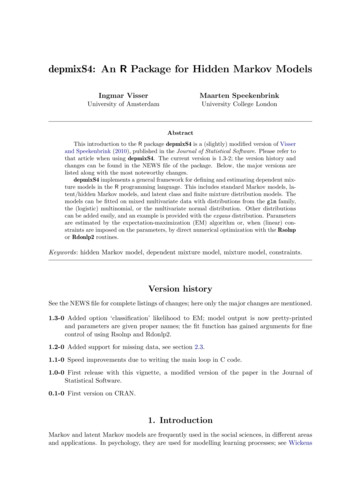
Ingmar Visser, Maarten Speekenbrink30.41.4rtcorr1.0prev1.8 0.0Pacc0.81.01.41.8 5.06.07.0Speed accuracy trade off050100150TimeFigure 1: Response times (rt), accuracy (corr) and pay-off values (Pacc) for the first series ofresponses in dataset speed.relative reward for speeded and/or accurate responding. These variables are measured on 168,134 and 137 occasions respectively (the first series of 168 trials is plotted in Figure 1). Thesedata are more fully described in Dutilh, Wagenmakers, Visser, and van der Maas (2011), andin the next section a number of example models for these data is described.The latent Markov model is usually associated with data of this type, in particular for multinomially distributed responses. However, commonly employed estimation procedures (e.g.,van de Pol et al. 1996), are not suitable for long time series due to underflow problems. Incontrast, the hidden Markov model is typically only used for ‘long’ univariate time series(Cappe et al. 2005, Chapter 1). We use the term “dependent mixture model” because one ofthe authors (Ingmar Visser) thought it was time for a new name to relate these models1 .The fundamental assumption of a dependent mixture model is that at any time point, theobservations are distributed as a mixture with n components (or states), and that timedependencies between the observations are due to time-dependencies between the mixturecomponents (i.e., transition probabilities between the components). These latter dependenciesare assumed to follow a first-order Markov process. In the models we are considering here,the mixture distributions, the initial mixture probabilities and transition probabilities can alldepend on covariates zt .In a dependent mixture model, the joint likelihood of observations O1:T and latent statesS1:T (S1 , . . . , ST ), given model parameters θ and covariates z1:T (z1 , . . . , zT ), can be1Only later he found out that Leroux and Puterman (1992) already coined the term dependent mixturemodels in an application with hidden Markov mixtures of Poisson count data.
4depmixS4: An R Package for Hidden Markov Modelswritten as:P(O1:T , S1:T θ, z1:T ) πi (z1 )bS1 (O1 z1 )TY 1aij (zt )bSt (Ot 1 zt 1 ),(1)t 1where we have the following elements:1. St is an element of S {1 . . . n}, a set of n latent classes or states.2. πi (z1 ) P(S1 i z1 ), giving the probability of class/state i at time t 1 with covariatez1 .3. aij (zt ) P(St 1 j St i, zt ), provides the probability of a transition from state i tostate j with covariate zt .4. bSt is a vector of observation densities bkj (zt ) P(Otk St j, zt ) that provide theconditional densities of observations Otk associated with latent class/state j and covariatezt , j 1, . . . , n, k 1, . . . , m.For the example data above, bkj could be a Gaussian distribution function for the responsetime variable, and a Bernoulli distribution for the accuracy variable. In the models consideredhere, both the transition probability functions aij and the initial state probability functionsπ may depend on covariates as well as the response distributions bkj .2.1. LikelihoodTo obtain maximum likelihood estimates of the model parameters, we need the marginallikelihood of the observations. For hidden Markov models, this marginal (log-)likelihoodis usually computed by the so-called forward-backward algorithm (Baum and Petrie 1966;Rabiner 1989), or rather by the forward part of this algorithm. Lystig and Hughes (2002)changed the forward algorithm in such a way as to allow computing the gradients of thelog-likelihood at the same time. They start by rewriting the likelihood as follows (for ease ofexposition the dependence on the model parameters and covariates is dropped here):LT P(O1:T ) TYP(Ot O1:(t 1) ),(2)t 1where P(O1 O0 ) : P(O1 ). Note that for a simple, i.e., observed, Markov chain these probabilities reduce to P(Ot O1 , . . . , Ot 1 ) P(Ot Ot 1 ). The log-likelihood can now be expressedas:TXlT log[P(Ot O1:(t 1) ].(3)t 1To compute the log-likelihood, Lystig and Hughes (2002) define the following (forward) recursion:φ1 (j) : P(O1 , S1 j) πj bj (O1 )nX[φt 1 (i)aij bj (Ot )] (Φt 1 ) 1 ,φt (j) : P(Ot , St j O1:(t 1) ) i 1(4)(5)
Ingmar Visser, Maarten Speekenbrink5Pwhere Φt ni 1 φt (i). Combining Φt P(Ot O1:(t 1) ), and equation (3) gives the followingexpression for the log-likelihood:TXlT log Φt .(6)t 12.2. Parameter estimationParameters are estimated in depmixS4 using the expectation-maximization (EM) algorithmor through the use of a general Newton-Raphson optimizer. In the EM algorithm, parametersare estimated by iteratively maximizing the expected joint log-likelihood of the parametersgiven the observations and states. Let θ (θ 1 , θ 2 , θ 3 ) be the general parameter vectorconsisting of three subvectors with parameters for the prior model, transition model, andresponse models respectively. The joint log-likelihood can be written as:log P(O1:T , S1:T z1:T , θ) log P(S1 z1 , θ 1 ) TXlog P(St St 1 , zt 1 , θ 2 )t 2 TXlog P(Ot St , zt , θ 3 ) (7)t 1This likelihood depends on the unobserved states S1:T . In the Expectation step, we replacethese with their expected values given a set of (initial) parameters θ 0 (θ 01 , θ 02 , θ 03 ) andobservations O1:T . The expected log-likelihood:Q(θ, θ 0 ) Eθ 0 (log P(O1:T , S1:T O1:T , z1:T , θ)),(8)can be written as:Q(θ, θ 0 ) nXγ1 (j) log P(S1 j z1 , θ 1 )j 1 T Xn XnXξt (j, k) log P(St k St 1 j, zt 1 , θ 2 )t 2 j 1 k 1 T Xn XmXγt (j) log P(Otk St j, zt , θ 3 ), (9)t 1 j 1 k 1where the expected values ξt (j, k) P (St k, St 1 j O1:T , z1:T , θ 0 ) and γt (j) P (St j O1:T , z1:T , θ 0 ) can be computed effectively by the forward-backward algorithm (see e.g.,Rabiner 1989). The Maximization step consists of the maximization of (9) for θ. As the righthand side of (9) consists of three separate parts, we can maximize separately for θ 1 , θ 2 and θ 3 .In common models, maximization for θ 1 and θ 2 is performed by the nnet.default routine inthe nnet package (Venables and Ripley 2002), and maximization for θ 3 by the standard glmroutine. Note that for the latter maximization, the expected values γt (j) are used as priorweights of the observations Otk .The EM algorithm however has some drawbacks. First, it can be slow to converge towardsthe end of optimization. Second, applying constraints to parameters can be problematic; in
6depmixS4: An R Package for Hidden Markov Modelsparticular, EM can lead to wrong parameter estimates when applying constraints. Hence, indepmixS4, EM is used by default in unconstrained models, but otherwise, direct optimizationis used. Two options are available for direct optimization using package Rsolnp (Ghalanosand Theußl 2010; Ye 1987), or Rdonlp2 (Tamura 2009; Spellucci 2002). Both packages canhandle general linear (in)equality constraints (and optionally also non-linear constraints).2.3. Missing dataMissing data can be dealt with straightforwardly in computing the likelihood using the forwardrecursion in Equations (4–5). Assume we have observed O1:(t 1) but that observation Ot ismissing. The key idea that, in this case, the filtering distribution, the probabilities φt , shouldbe identical to the state prediction distribution, as there is no additional information toestimate the current state. Thus, the forward variables φt are now computed as:φt (i) P(St i O1:(t 1) )nX φt 1 (j)P(St i St 1 j).(10)(11)j 1For later observations, we can then use this latter equation again, realizing that the filteringdistribution is technically e.g. P(St 1 O1:(t 1),t 1 ). Computationally, the easiest way toimplement this is to simply set b(Ot St ) 1 if Ot is missing.3. Using depmixS4Two steps are involved in using depmixS4 which are illustrated below with examples:1. model specification with function depmix (or with mix for latent class and finite mixturemodels, see example below on adding covariates to prior probabilities);2. model fitting with function fit.We have separated the stages of model specification and model fitting because fitting largemodels can be fairly time-consuming and it is hence useful to be able to check the modelspecification before actually fitting the model.3.1. Example data: speedThroughout this article a data set called speed is used. As already indicated in the introduction, it consists of three time series with three variables: response time rt, accuracy corr, anda covariate, Pacc, which defines the relative pay-off for speeded versus accurate responding.Before describing some of the models that are fitted to these data, we provide a brief sketchof the reasons for gathering these data in the first place.Response times are a very common dependent variable in psychological experiments andhence form the basis for inference about many psychological processes. A potential threat tosuch inference based on response times is formed by the speed-accuracy trade-off: differentparticipants in an experiment may respond differently to typical instructions to ‘respond asfast and accurate as possible’. A popular model which takes the speed-accuracy trade-off
Ingmar Visser, Maarten Speekenbrink7into account is the diffusion model (Ratcliff 1978), which has proven to provide accuratedescriptions of response times in many different settings.One potential problem with the diffusion model is that it predicts a continuous trade-offbetween speed and accuracy of responding, i.e., when participants are pressed to respondfaster and faster, the diffusion model predicts that this would lead to a gradual decrease inaccuracy. The speed data set that we analyze below was gathered to test this hypothesisversus the alternative hypothesis stating that there is a sudden transition from slow andaccurate responding to fast responding at chance level. At each trial of the experiment, theparticipant is shown the current setting of the relative reward for speed versus accuracy. Thebottom panel of Figure 1 shows the values of this variable. The experiment was designed toinvestigate what would happen when this reward variable changes from reward for accuracyonly to reward for speed only. The speed data that we analyse here are from participant A inExperiment 1 in Dutilh et al. (2011), who provide a complete description of the experimentand the relevant theoretical background.The central question regarding this data is whether it is indeed best described by two modesof responding rather than a single mode of responding with a continuous trade-off betweenspeed and accuracy. The hallmark of a discontinuity between slow versus speeded respondingis that switching between the two modes is asymmetric (see e.g. Van der Maas and Molenaar1992, for a theoretical underpinning of this claim). The fit help page of depmixS4 provides anumber of examples in which the asymmetry of the switching process is tested; those examplesand other candidate models are discussed at length in Visser, Raijmakers, and Van der Maas(2009).3.2. A simple modelA dependent mixture model is defined by the number of states and the initial state, statetransition, and response distribution functions. A dependent mixture model can be createdwith the depmix function as follows:R R R R library("depmixS4")data("speed")set.seed(1)mod - depmix(response rt 1, data speed, nstates 2,trstart runif(4))The first line of code loads the depmixS4 package and data(speed) loads the speed data set.The line set.seed(1) is necessary to get starting values that will result in the right model,see more on starting values below.The call to depmix specifies the model with a number of arguments. The response argumentis used to specify the response variable, possibly with covariates, in the familiar format usingformulae such as in lm or glm models. The second argument, data speed, provides thedata.frame in which the variables from response are interpreted. Third, the number ofstates of the model is given by nstates 2.Starting values. Note also that start values for the transition parameters are provided inthis call by the trstart argument. Starting values for parameters can be provided using
8depmixS4: An R Package for Hidden Markov Modelsthree arguments: instart for the parameters relating to the prior probabilities, trstart,relating the transition models, and respstart for the parameters of the response models.Note that the starting values for the initial and transition models as well as multinomial logitresponse models are interpreted as probabilities, and internally converted to multinomial logitparameters (if a logit link function is used). Start values can also be generated randomlywithin the EM algorithm by generating random uniform values for the values of γt in (9) atiteration 0. Automatic generation of starting values is not available for constrained models(see below). In the call to fit below, the argument emc em.control(rand FALSE) controlsthe EM algorithm and specifies that random start values should not be generated2 .Fitting the model and printing results. The depmix function returns an object of class‘depmix’ which contains the model specification, and not a fitted model. Hence, the modelneeds to be fitted by calling fit:R fm - fit(mod, emc em.control(rand rationiterationiterationiterationconverged0 logLik: -305.35 logLik: -305.310 logLik: -305.315 logLik: -305.320 logLik: -305.325 logLik: -305.330 logLik: -305.335 logLik: -305.340 logLik: -305.145 logLik: -304.550 logLik: -276.755 logLik: -89.8360 logLik: -88.7365 logLik: -88.73at iteration 68 with logLik: -88.73The fit function returns an object of class ‘depmix.fitted’ which extends the ‘depmix’ class,adding convergence information (and information about constraints if these were applied, seebelow). The class has print and summary methods to see the results. The print methodprovides information on convergence, the log-likelihood and the AIC and BIC values:R fmConvergence info: Log likelihood converged to within tol. (relative change)'log Lik.' -88.73 (df 7)AIC: 191.5BIC: 220.1These statistics can also be extracted using logLik, AIC and BIC, respectively. By comparison, a 1-state model for these data, i.e., assuming there is no mixture, has a log-likelihood of2As of version 1.0-1, the default is have random parameter initialization when using the EM algorithm.
Ingmar Visser, Maarten Speekenbrink9 305.33, and 614.66, and 622.83 for the AIC and BIC respectively. Hence, the 2-state modelfits the data much better than the 1-state model. Note that the 1-state model can be specified using mod - depmix(rt 1, data speed, nstates 1), although this model istrivial as it will simply return the mean and standard deviation of the rt variable.The summary method of fitted models provides the parameter estimates, first for the priorprobabilities model, second for the transition models, and third for the response models.R summary(fm)Initial state probabilties modelpr1 pr210Transition matrixtoS1toS2fromS1 0.9157 0.08433fromS2 0.1165 0.88351Response parametersResp 1 : gaussianRe1.(Intercept) Re1.sdSt16.385 0.2442St25.510 0.1918Since no further arguments were specified, the initial state, state transition and responsedistributions were set to their defaults (multinomial distributions for the first two, and aGaussian distribution for the response). The resulting model indicates two well-separatedstates, one with slow and the second with fast responses. The transition probabilities indicaterather stable states, i.e., the probability of remaining in either of the states is around 0.9. Theinitial state probability estimates indicate that state 1 is the starting state for the process,with a negligible probability of starting in state 2.3.3. Covariates on transition parametersBy default, the transition probabilities and the initial state probabilities are parameterizedusing a multinomial model with an identity link function. Using a multinomial logistic modelallows one to include covariates on the initial state and transition probabilities. In this case,each row of the transition matrix is parameterized by a baseline category logistic multinomial,meaning that the parameter for the base category is fixed at zero (see Agresti 2002, p. 267 ff.,for multinomial logistic models and various parameterizations). The default baseline category is the first state. Hence, for example, for a 3-state model, the initial state probabilitymodel would have three parameters of which the first is fixed at zero and the other two arefreely estimated. Chung, Walls, and Park (2007) discuss a related latent transition model forrepeated measurement data (T 2) using logistic regression on the transition parameters;they rely on Bayesian methods of estimation. Covariates on the transition probabilities canbe specified using a one-sided formula as in the following example:
10depmixS4: An R Package for Hidden Markov ModelsR set.seed(1)R mod - depmix(rt 1, data speed, nstates 2, family gaussian(), transition scale(Pacc), instart runif(2))R fm - fit(mod, verbose FALSE, emc em.control(rand FALSE))converged at iteration 42 with logLik: -44.2Note the use of verbose FALSE to suppress printing of information on the iterations of thefitting process. Applying summary to the fitted object gives (only transition models printedhere by using argument which):R summary(fm, which "transition")Transition model for state (component) 1Model of type multinomial (mlogit), formula: scale(Pacc)Coefficients:St1St2(Intercept)0 -0.9518scale(Pacc)0 1.3924Probalities at zero values of the covariates.0.7215 0.2785Transition model for state (component) 2Model of type multinomial (mlogit), formula: scale(Pacc)Coefficients:St1St2(Intercept)0 2.472scale(Pacc)0 3.581Probalities at zero values of the covariates.0.07788 0.9221The summary provides all parameters of the model, also the (redundant) zeroes for the baseline category in the multinomial model. The summary also prints the transition probabilitiesat the zero value of the covariate. Note that scaling of the covariate is useful in this regardas it makes interpretation of these intercept probabilities easier.3.4. Multivariate dataMultivariate data can be modelled by providing a list of formulae as well as a list of familyobjects for the distributions of the various responses. In above examples we have only usedthe response times which were modelled as a Gaussian distribution. The accuracy variable inthe speed data can be modelled with a multinomial by specifying the following:R set.seed(1)R mod - depmix(list(rt 1,corr 1), data speed, nstates 2, family list(gaussian(), multinomial("identity")), transition scale(Pacc), instart runif(2))R fm - fit(mod, verbose FALSE, emc em.control(rand FALSE))
Ingmar Visser, Maarten Speekenbrink11converged at iteration 31 with logLik: -255.5This provides the following fitted model parameters (only the response parameters are givenhere):R summary(fm, which "response")Response parametersResp 1 : gaussianResp 2 : multinomialRe1.(Intercept) Re1.sd Re2.pr1 Re2.pr2St15.517 0.1974 0.4747 0.5253St26.391 0.2386 0.0979 0.9021As can be seen, state 1 has fast response times and accuracy is approximately at chance level(.4747), whereas state 2 corresponds with slower responding at higher accuracy levels (.9021).Note that by specifying multivariate observations in terms of a list, the variables are considered conditionally independent (given the states). Conditionally dependent variables mustbe handled as a single element in the list. Effectively, this means specifying a multivariate response model. Currently, depmixS4 has one multivariate response model which is formultivariate normal variables.3.5. Fixing and constraining parametersUsing package Rsolnp (Ghalanos and Theußl 2010) or Rdonlp2 (Tamura 2009), parametersmay be fitted subject to general linear (in-)equality constraints. Constraining and fixingparameters is done using the conpat argument to the fit function, which specifies for eachparameter in the model whether it’s fixed (0) or free (1 or higher). Equality constraints canbe imposed by giving two parameters the same number in the conpat vector. When only fixedvalues are required, the fixed argument can be used instead of conpat, with zeroes for fixedparameters and other values (e.g., ones) for non-fixed parameters. Fitting the models subjectto these constraints is handled by the optimization routine solnp or, optionally, by donlp2.To be able to construct the conpat and/or fixed vectors one needs the correct ordering ofparameters which is briefly discussed next before proceeding with an example.Parameter numbering. When using the conpat and fixed arguments, complete parameter vectors should be supplied, i.e., these vectors should have length equal to the number ofparameters of the model, which can be obtained by calling npar(object). Note that this isnot the same as the degrees of freedom used e.g., in the logLik function because npar alsocounts the baseline category zeroes from the multinomial logistic models. Parameters arenumbered in the following order:1. the prior model parameters;2. the parameters for the transition models;3. the response model parameters per state (and subsequently per response in the case ofmultivariate time series).
12depmixS4: An R Package for Hidden Markov ModelsTo see the ordering of parameters use the following:R setpars(mod, value 1:npar(mod))To see which parameters are fixed (by default only baseline parameters in the multinomiallogistic models for the transition models and the initial state probabilities model):R setpars(mod, getpars(mod, which "fixed"))When fitting constraints it is useful to have good starting values for the parameters and hencewe first fit the following model without constraints:R trst - c(0.9, 0.1, 0, 0, 0.1, 0.9, 0, 0)R mod - depmix(list(rt 1,corr 1), data speed, transition Pacc, nstates 2, family list(gaussian(), multinomial("identity")), trstart trst, instart c(0.99, 0.01))R fm1 - fit(mod,verbose FALSE, emc em.control(rand FALSE))converged at iteration 23 with logLik: -255.5After this, we use the fitted values from this model to constrain the regression coefficients onthe transition matrix (parameters number 6 and 10):R R R R R R R R R pars - c(unlist(getpars(fm1)))pars[6] - pars[10] - 11pars[1] - 0pars[2] - 1pars[13] - pars[14] - 0.5fm1 - setpars(mod, pars)conpat - c(0, 0, rep(c(0, 1), 4), 1, 1, 0, 0, 1, 1, 1, 1)conpat[6] - conpat[10] - 2fm2 - fit(fm1, equal conpat)Using summary on the fitted model shows that the regression coefficients are now estimated atthe same value of 12.66. Setting elements 13 and 14 of conpat to zero resulted in fixing thoseparameters at their starting values of 0.5. This means that state 1 can now be interpretedas a ’guessing’ state which is associated with comparatively fast responses. Similarly forelements 1 and 2, resulting in fixed initial probabilities. The function llratio computes thelikelihood ratio χ2 -statistic and the associated p-value with appropriate degrees of freedom fortesting the tenability of constraints; Giudici, Ryden, and Vandekerkhove (2000) shows thatthe ‘standard asymptotic theory of likelihood-ratio tests is valid’ in hidden Markov models.(Dannemann and Holzmann 2007) discusses extension to non-standard situations, e.g. fortesting parameters on the boundary. Note that these arguments (i.e., conpat and conrows)provide the possibility for arbitrary constraints, also between, e.g., a multinomial regressioncoefficient for the transition matrix and the mean of a Gaussian response model. Whethersuch constraints make sense is hence the responsibility of the user.
Ingmar Visser, Maarten Speekenbrink13Figure 2: Balance scale item; this is a distance item (see the text for details).3.6. Adding covariates on the prior probabilitiesTo illustrate the use of covariates on the prior probabilities we have included another data setwith depmixS4. The balance data consists of 4 binary items (correct-incorrect) on a balancescale task (Siegler 1981). The data form a subset of the data published in Jansen and van derMaas (2002). Before specifying specifying a model for these data, we briefly describe them.The balance scale task is a famous task for testing cognitive strategies developed by JeanPiaget (see Siegler 1981). Figure 2 provides an example of a balance scale item. Parti
expression for the log-likelihood: l T XT t 1 log t: (6) 2.2. Parameter estimation Parameters are estimated in depmixS4 using the expectation-maximization (EM) algorithm or through the use of a general Newton-Raphson optimizer. In the EM algorithm, parameters are estimated by iteratively maximizing the expected joint log-likelihood of the .