Transcription
PRACTICAL ALGORITHMS FOR LEARNING NEAR-ISOMETRICLINEAR EMBEDDINGS JERRY LUO† , KAYLA SHAPIRO‡ , HAO-JUN MICHAEL SHI§ , QI YANG¶, AND KANZHUkAbstract. We propose two practical non-convex approaches for learning near-isometric, linearembeddings of finite sets of data points. Given a set of training points X , we consider the secant setS(X ) that consists of all pairwise difference vectors of X , normalized to lie on the unit sphere. Theproblem can be formulated as finding a symmetric and positive semi-definite matrix Ψ that preservesthe norms of all the vectors in S(X ) up to a distortion parameter δ. Motivated by non-negativematrix factorization, we reformulate our problem into a Frobenius norm minimization problem, whichis solved by the Alternating Direction Method of Multipliers (ADMM) and develop an algorithm,FroMax. Another method solves for a projection matrix Ψ by minimizing the restricted isometryproperty (RIP) directly over the set of symmetric, postive semi-definite matrices. Applying ADMMand a Moreau decomposition on a proximal mapping, we develop another algorithm, NILE-Pro,for dimensionality reduction. FroMax is shown to converge faster for smaller δ while NILE-Proconverges faster for larger δ. Both non-convex approaches are then empirically demonstrated to bemore computationally efficient than prior convex approaches for a number of applications in machinelearning and signal processing.Key words. dimensionality reduction, linear embeddings, compressive sensing, approximatenearest neighbors, classification1. Introduction.1.1. Motivation. The size of the acquired raw data currently poses a challenge to current state-of-the-art information processing systems. Since many machinelearning algorithms’ computational efficiency scale with the complexity of the data,machine learning researchers have introduced a family of algorithms for dimensionality reduction to address this issue. Dimensionality reduction algorithms constructa concise representation of high-dimensional data on a lower-dimensional subspace,with as minimal loss of intrinsic information as possible. This representation is oftenreferred to as a low-dimensional embedding.The canonical approach in statistics for constructing a linear embedding is principal components analysis (PCA) [14]. PCA is a linear embedding technique thatprojects data points onto a lower-dimensional subspace spanned by the principal components that contain the most variability within the data. PCA benefits from beingcomputationally efficient and easily generalizable to new data sets; however, it failsto preserve pairwise distances between sample data points, sometimes rendering twodistinct points indistinguishable in the low-dimensional embedding space. This canpotentially hamper the performance of PCA and other similar algorithms. This research was conducted as part of the California Research Training Program in Computational and Applied Mathematics 2014.† Department of Mathematics,University of Arizona, Tucson, AZ 85721.(jerryluo@math.arizona.edu)‡ Department of Computing, Imperial College London, London SW7 2AZ, United Kingdom.(k.shapiro@berkeley.edu)§ Department of Mathematics, University of California, Los Angeles, Los Angeles, CA 90024.(hjmshi@ucla.edu)¶ Department of Mathematics, University of Southern California, Los Angeles, 90089.(yangq@usc.edu)k Departmentof Computer Science, Columbia University, New York, NY 10027.(kzhu9@ucla.edu)Copyright SIAMUnauthorized reproduction of this article is prohibited178
Other popular nonlinear, manifold learning methods, such as ISOMAP and locallylinear embedding (LLE), preserve geometric structure by approximating geodesicsfrom k-nearest neighbors. Although these methods produce embeddings which areeasy to explicitly store and generalize, most fail to preserve all pairwise distancesbetween data points.A linear embedding technique that preserves all pairwise distances is the methodof random projections. Given X , a cloud of Q data points in a high-dimensional Euclidean space RN , the Johnson-Lindenstrauss Lemma [8] states that there exists a linear, near-isometric, or distance preserving, embedding such that X can be mapped toa subspace of dimension M O(log Q) with high probability. Despite its conceptualsimplicity, random projections suffers from probabilistic and asymptotic theoreticalguarantees in Johnson-Lindenstrauss [8]. A random projections mapping is also independent of the data under consideration, failing to utilize the geometric structureof the data.We would like to deterministically devise a linear embedding for dimensionalityreduction that preserves all normalized pairwise distances. In particular, linear embeddings can be explicitly stored using a matrix operator and can therefore be quicklyapplied to any new data point.1.2. Related Work. Using the geometric structure of the data, Hegde, et. al.developed a new deterministic approach, NuMax, to construct a near-isometric, linearembedding [6]. Given a training set X RN , the secant set is constructed by taking allpairwise difference vectors of X , which are then normalized to lie on the unit sphere.Hegde, et. al. formulated a rank minimization problem with affine constraints toconstruct a projection matrix ψ that preserves norms of all vectors in S(X ) up toa distortion parameter δ. They then relax this problem to a convex program thatcan be solved using a tractable semidefinite program (SDP), with column generationfor large data sets, and develop NuMax based on the Alternating Direction Methodof Multipliers (ADMM). This framework deterministically produces a near-isometriclinear embedding. Other algorithmic approaches for finding near-isometric linearembeddings are also described in [4, 5, 19].1.3. Organization. The rest of the paper is organized as follows. We review therestricted isometry property and NuMax algorithm in §2. The FroMax algorithm isintroduced in §3. NILE-Pro is discussed in §4. Rank adjustment and column generation methods which increase computational efficiency for large data sets is introducedin §5. Numerical simulations and runtime performance results are presented in §7.Lastly, §8 concludes the paper and gives direction for future work.2. Background.2.1. Restricted Isometry Property (RIP). E. Candes, et. al. introduced aformal, relaxed notion of isometry in [1] as follows:Definition 2.1. Suppose M N and consider X RN . An embedding operatorP : X RM satisfies the restricted isometry property (RIP) on X if there exists apositive constant δ 0 such that, for every x, x0 X , the following relation holds:(2.1)(1 δ)kx x0 k22 kPx Px0 k22 (1 δ)kx x0 k22 .We may also refer to δ as the isometry constant. Intuitively, this notion of nearisometry requires the distance of every pair of points in X to be almost preserved.179
Hegde, et. al. [6] leveraged this idea to develop a framework for finding low rankmatrices that satisfy the RIP.2.2. NuMax. In this section, we review Hegde et. al. [6]’s work on NuMax.Given a data set X RN , Hegde et. al. formulate the secant set as follows: x x000(2.2)S(X ) ,x,x X,x 6x.kx x0 k2Hegde, et. al. seeks to find a projection matrix Ψ RM N with the smallest possiblerank that satisfies the RIP on S(X ) for a given δ 0. This problem is then cast asan optimization problem over all symmetric matrices which we denote as SN N . LetP ΨT Ψ SN N with rank(P) M . Then for all secants vi S(X ), we mayrewrite the RIP constraint as:(2.3)(1 δ)kvi k22 kΨvi k22 (1 δ)kvi k22 .After grouping we get:(2.4) kΨvi k22 kvi k22 δkvi k22 .Then we isolate δ and use the fact that kΨvi k22 viT Pvi :(2.5) kΨvi k22 1 δ(2.6) viT Pvi 1 δ.Let 1S denote the S-dimensional ones vector and A : RN N RS where S S(X ) ,and A : X 7 {viT Xvi }Si 1 , where the output is understood to be an S dimensionalvector with the i-th entry being viT Xvi . This admits the rank minimization problem:minimizeP(2.7)rank(P)subject to kA(P) 1S k δP 0.Here, P 0 means P is symmetric positive semidefinite. However, since rank minimization is a non-convex, NP-hard problem [16], a convex relaxation is performed onthe objective to obtain the following nuclear-norm minimization:minimizeP(2.8)kPk subject to kA(P) 1S k δP 0,where kPk is the nuclear norm of P, or the sum of the singular values of P. Thenthe desired linear embedding Ψ RM N can be found by taking a matrix squareroot of the minimizer P UΓUT by(2.9)1/2Ψ ΓM UTM ,where ΓM diag{λ1 , ., λM } denotes the M leading (non-zero) eigenvalues of P and UM are the corresponding eigenvectors.180
Applying the Alternating Direction Method of Multipliers (ADMM), the optimization problem is rewritten by introducing auxiliary variables L SN N andq RS :minimizeP,L,q(2.10)kPk subject to P LA(L) q,kq 1S k δP 0.Introducing auxiliary variables L and q allows constrained optimization techniquesto be applied while breaking up the problem into simpler subproblems. The linearconstraints are then relaxed to form an augmented Lagrangian as follows:(2.11)LA (P, L, q; Γ, ω) kPk β1β2kP L Γk2F kA(L) q ωk22 ,22where Γ SN N and ω RS represent the scaled Lagrange multipliers and β1 , β2 Rare chosen parameters.NuMax then solves the following augmented Lagrangian problem:minimizeP,L,q,Γ,ω(2.12)LA (P, L, q, Γ, ω)subject to kq 1S k δP 0,P, L and q are optimized in an alternating fashion, i.e. optimized one at a timewith the others held fixed. This optimization can then be solved by three easiersub-problems, admitting a computationally efficient solution.For more information regarding theoretical and empirical properties of NuMax,please refer to Hegde et. al. [6].This framework, though slower than conventional methods such as PCA andrandom projections, deterministically admits a projection matrix satisfying the RIPwith low rank. However, NuMax computes a singular value decomposition of P eachiteration, which is computationally expensive. Furthermore, though minimizing thenuclear-norm tends to give low rank matrices, NuMax does not theoretically guaranteethe lowest rank embedding for a given δ.These issues motivate the pursuit of other practical algorithms that optimize similar non-convex problems that may admit low rank, near-isometric projection matricesthat give faster, but sufficient (not necessarily optimal) results. Rather than solvingboth the rank minimization and near-isometry problems simultaneously, we solve asimpler non-convex problem quickly to find a near-isometric projection matrix andapply a rank adjustment heuristic to choose a minimal rank.3. FroMax. Our first algorithm, Frobenius norm minimization with Max-normconstraints, or FroMax, combines ideas from NuMax and NMF to formulate a Frobenius norm minimization problem which we then solve based on ADMM, similar toNuMax [22]. Though this algorithm does not discover the optimal rank for Ψ, wecombine FroMax with a rank adjustment heuristic to find low rank embeddings.181
3.1. Non-Negative Matrix Factorization (NMF). FroMax is motivatedby ideas from non-negative matrix factorization. Non-negative matrix factorization(NMF) is a group of algorithms that factorize a non-negative matrix V into two lowrank non-negative matrices W and H [12]. More rigorously, let V RN M be given,then we solve for W RM Q , and H RQ N by solving the following optimizationproblem:minimize(3.1)W,HkWH Vk2Fsubject to Wij 0, Hij 0, i, j.NMF motivates the problem formulation for our first algorithm, FroMax.3.2. Optimization Framework. We formulate a specialized matrix factorization minimization problem to solve for a near-isometric linear embedding as follows:Given a desired rank r N , let Ψ Rr N be the variable projection matrix. Here,we seek to solve:(3.2)1kP ΨT Ψk2F2subject to kA(P) 1S k δ,minimizeP,Ψwhere P RN N is a variable.We introduce auxiliary variables to simplify our optimization and break up ourproblem into simpler subproblems that can be solved by applying ADMM. In particular, let Y Ψ Rr N , X YT RN r . Then1kP XYk2F2subject to A(P) qminimizeP,X,Y,q(3.3)Y XTkq 1S k δ.This gives Y Ψ Rr N such that the RIP holds for all secant vectors in thesecant set S(X ) for an isometry constant δ. The optimization formulation for (3.2) isconceptually simple, only requiring the input data set X , desired isometry constantδ 0 and desired rank r.An important caveat is that our optimization problem is non-convex. Thus, wecannot guarantee that FroMax will converge to the optimal solution of (3.2). However,various experiments in §7 indicate that FroMax yields excellent, stable results for realworld data sets and finds projection matrices faster than NuMax and other convexapproaches. We implement ADMM since Wang et. al. [21] indicate that ADMMis more likely to converge than the Augmented Lagrangian Method for nonconvex,nonsmooth problems.3.3. ADMM. We develop our algorithm, FroMax, to solve (3.3) based on ADMM.We relax the linear constraints and form an augmented Lagrangian of (3.3) as follows:(3.4) LA (X, Y, q, P) 1kP XYk2F λT (A(P) q) hΓ, Y XT i2β1β2 kA(P) qk22 kY XT k2F ι{q:kq 1S k δ} .22182
Here, λ RN and Γ Rr N represent the scaled Lagrange multipliers. The indicatorfunction, ι{q:kq 1S k δ} , is defined as(0if kq 1S k δι{q:kq 1S k δ} otherwise.The optimization in (3.4) is carried out over P RN N , X RN r , Y Rr N ,and q RS , while λ and Γ are also iteratively updated. We optimize each variablein an alternating fashion like NuMax. The following steps below are performed untilconvergence.Update q: Isolating the terms that involve q, we obtain a new estimate qk 1 asthe solution of the constrained optimization problem(3.5)qk 1 arg min λTk (A(Pk ) q) qβ1kA(Pk ) qk22 ι{q:kq 1S k δ} .2Define z A(Pk ) λk 1S . Using a component-wise truncation procedure for entriesin q, we easily see thatqk 1 1S sign(z) · min( z , δ),(3.6)where the sign and min operators are applied component-wise.Update P: Isolating the terms that involve P, we obtain a new estimate Pk 1as the solution of the constrained optimization problem(3.7) Pk 1 arg minPβ11kP Xk Yk k2F λTk (A(P) qk 1 ) kA(P) qk 1 k22 ,22such that P 0. Since this is a least-squares problem, we can solve for the minimumby solving:(3.8)(P Xk Yk ) SXλk,j vj vjT β1 A (A(P) qk 1 ) 0,j 1where A is the adjoint of A. The solution is(3.9) † Pk 1 (I β1 A A) (β1 A qk 1 Xk Yk sXλk,j vj vjT )j 1where † denotes the pseudoinverse.Update X: Isolating the terms that involve X, we obtain a new estimate Xk 1as the solution of the constrained optimization problem(3.10)Xk 1 arg minX1β2kPk 1 XYk k2F hΓk , Yk XT i kYk XT k2F .22It is easily seen that this can be solved similarly to the P update.Update Y: Isolating the terms that involve Y, we obtain a new estimate Yk 1as the solution of the constrained optimization problem(3.11) Yk 1 arg minY1β2kPk 1 Xk 1 Yk2F hΓk , Y XTk 1 i kY XTk 1 k2F .22183
Algorithm 1 FroMaxInputs: Secant set S(X ) {vi }Si 1 , isometry constant δ, desired rank for P r,max iterations m 0Parameters: β1 , β2 , η 0Output: P, X, Yfor k 1 to m doz A(Pk ) λk 1Sqk 1 1S sign(z) · min( z , δ)Pk 1 (I β1 A A)† (β1 A qk 1 Xk Yk Psj 1λk,j vj vjT )Xk 1 (ΓTk β2 YkT Pk 1 YkT )(Yk YkT β2 I) 1Yk 1 (XTk 1 Xk 1 β2 I) 1 (XTk 1 Pk 1 Γk β2 XTk 1 )λk 1 λk ηβ1 (A(Pk 1 ) qk 1 )Γk 1 Γk ηβ2 (Yk 1 XTk 1 )122 kPk 1 Xk 1 Yk 1 kF thenbreakend ififend forreturn P Pk , X Xk , Y YkIt is easily seen that this can be solved similarly to the X update.Update λ, Γ: Following standard augmented Lagrangian methods, we updateΓ, Π according to the following equations(3.12)λk 1 λk ηβ1 (A(Pk 1 ) qk 1 )(3.13)Γk 1 Γk ηβ2 (Yk 1 XTk 1 ).Pseudocode for FroMax may be found in Algorithm 1. Convergence properties ofFroMax are highly dependent on chosen parameters η, β1 , and β2 .4. NILE-Pro. Our second algorithm, Near-Isometric Linear Embedding via Proximal Mapping, or NILE-Pro seeks to minimize the RIP constraint directly to solve forΨ. This minimization problem is solved using ADMM and a Moreau decompositionon a proximal mapping.4.1. Optimization Framework. We formulate a new framework for NILE-Pro.We solve for our desired linear embedding Ψ directly:(4.1)minimize kA(ΨT Ψ) 1S k .ΨBy introducing an auxiliary variable q, which simplifies our problem and allows usto apply constrained optimization techniques, we then have the following minimization184
problem:minimize kq 1S k (4.2)q,Ψsubject to q A(ΨT Ψ).We apply ADMM and use a Moreau decomposition on a proximal mapping to solve forupdates. Like FroMax, this optimization problem is non-convex and thus, we cannotguarantee that NILE-Pro will converge to the optimal solution of (4.1). However, wedemonstrate in §7 that NILE-Pro may produce stable, excellent results for syntheticand real-world data sets at a much faster rate than both FroMax and NuMax due tothe simplified problem it solves.4.2. Proximal Mapping and Moreau Decomposition. We introduce somemachinery to solve this minimization problem:Definition 4.1. The proximal mapping [17] of a closed proper convex functionf is defined to be1proxf (x) arg min(f (u) ku xk22 ).2uThe proximal mapping may be interpreted as a compromise between minimizingf and staying near the original iterate x. Proximal mappings generalize projections,and are particularly useful since they often work very fast in practice.Theorem 4.2. If a function f : Rn R is proper, closed, and convex, thenproxf (x) exists, well-defined, and unique for all x [17].This theorem guarantees that these proximal mappings exist for closed, proper,and convex functions.Definition 4.3. The convex conjugate [17] of a closed proper convex function fis defined to bef (y) sup(yT x f (x)).xThen for any x, the following relation holds:x proxf (x) proxf (x),where f is the convex conjugate of f . This decomposition, called the Moreau decomposition, generalizes the orthogonal decomposition on subspaces. We apply thismachinery to help us solve for the update for q.4.3. ADMM. Following a similar method as FroMax, we relax our linear constraints and find our augmented Lagrangian of (14):(4.3)LA (Ψ, q; ω) kq 1S k βkA(ΨT Ψ) q ωk22 .2Here, ω RS is the scaled Lagrange multiplier. The optimization in (4.3) is carriedout over Ψ Rr N and q RS , while ω is updated. Each variable is updated in analternating fashion. The following steps below are performed until convergence.185
Update Ψ: Isolating the terms that involve Ψ, we obtain a new estimate Ψk 1as the solution of the constrained optimization problem(4.4)Ψk 1 arg minΨβkA(ΨT Ψ) qk ω k k22 .2Update q: Isolating the terms that involve q, we obtain a new estimate qk 1 asthe solution of the constrained optimization problem(4.5)qk 1 arg min kq 1S k qβkA(ΨTk 1 Ψk 1 ) q ω k k22 .2Set x qk 1 1S and τ A(ΨTk 1 Ψk 1 ) ω k 1S , let f (x) convex conjugate 0 if kβxk1 1 f (x) . if kβxk1 11β kxk and itsThen proxf (τ ) P{kxk1 1} (βτ ), i.e. the projection of βτ to the 1 ball. Thenapplying Moreau’s decomposition, we have the q update:(4.6)(4.7)1(βτ P{kxk1 1} (βτ ))β1q (βτ P{kxk1 1} (βτ )) 1S .βx Update ω: Following standard augmented Lagrangian methods, we update ωaccording to the following equation(4.8)ω k 1 ω k β(A(ΨTk 1 Ψk 1 ) qk 1 ).Pseudocode for NILE-Pro may be found in Algorithm 2.5. Rank Adjustment and Column Generation. In this section, we discussrank adjustment and column generation heuristics. We develop rank adjustmentmethods to discover the lowest optimal rank for both FroMax and NILE-Pro. Abbreviating rank adjustment to RA, we call our rank adjusted algorithms FroMax RAand NILE-Pro RA, respectively. We also use column generation techniques followingHegde et. al. [6] to work with subsets of S(X ) to lower the memory complexity ofthese algorithms, which we name FroMax CG and NILE-Pro CG, respectively. Wediscuss each heuristic algorithm in detail below.5.1. Rank Adjustment. Though FroMax and NILE-Pro may dramatically decrease the time of solving for projection matrix Ψ, both algorithms do not find anoptimal rank for dimensionality reduction like NuMax. Hence, we propose a heuristicrank adjustment method that uses the discovered matrix P ΨT Ψ to give a goodinitialization for Ψ of lower rank.Given a sufficiently large rank, R0 r, the optimal rank, we run our dimensionality reduction algorithm for a maximum number of iterations or until convergence1/2to find Ψ. If our algorithm converges, we return P ΨT Ψ and find Ψ0 ΓM UTM ,Twhere P UΓU from P’s eigendecomposition. We then initialize our algorithmagain with rank R1 R0 1 and Ψ0 which we found in the last iteration and testagain for convergence. We continue this process until we reach the maximum numberof iterations within the algorithm and return the Ψ given in the last iteration, considering its rank r Rk to be optimal. We summarize our rank adjustment heuristicin Algorithm 3.186
Algorithm 2 NILE-ProInputs: Secant set S(X ) {vi }Si 1 , isometry constant δ, max iterations m 0,initial rank rParameters: β 0Output: Ψfor k 1, ., m doτ A(ΨTk Ψk ) ω 1s qk 1 β1 βτ P{kxk1 1} (βτ ) 1SΨk 1 Ψk 2ηΨk A (A(ΨTk Ψk ) qk 1 ω)ω k 1 ω k β(A(ΨTk 1 Ψk 1 ) qk 1 ) 0 kA(ΨTk 1 Ψk 1 ) 1S k if 0 thenbreakend ifend forreturn Ψ ΨkAlgorithm 3 FroMax/NILE-Pro RAInputs: Secant set S(X ) {vi }Si 1 , isometry constant δ, max iterations for algorithm m 0, initial rank R0 , max iterations for RA M , Ψ0for k 1, ., M doΨ FroMax/NILE-Pro(S, δ, m, R0 , Ψ0 )P ΨT ΨRk 1 Rk 1[Γ, U ] eig(P )Ψ0 Γ1/2 U Tif FroMax/NILE-Pro does not converge thenbreakend ifend forreturn Ψ, r Rk5.2. Column Generation. Since FroMax and NILE-Pro use the secants of agiven data set, applications involving millions of secants may be prohibited by thememory complexity of these algorithms. Some methods that are used to addresslarge data sets include stochastic and online methods. Stochastic methods use random subsets of the data to learn an estimate for the entire data set [9, 20]. Onlinemethods uses sequentially available data to update the current iterate then discardsthe information [13, 10]. Our column generation algorithms, FroMax CG and NILE-187
Algorithm 4 FroMax/NILE-Pro CGInputs: Secant set S(X ) {vi }Si 1 , isometry constant δ, max iterations for algorithm m 0, rank r, the FroMax or NILE-Pro algorithmwhile not converged doSb {vi S0 : viT ΨT Ψvi 1 δ}00S1 {vi S(X ) : vi / S0 }Si 1STSb Sb {vi S1 : viT Ψ Ψvi 1 δ}b δ)Ψ FroMax/NILE-Pro(S,bS0 Send whilereturn ΨPro CG, combines stochastic and online methods to estimate solutions to large-scaleproblems.Similar to NuMax’s column generation, which is based off of the Karush-KuhnTucker (KKT) conditions, we apply a simple, greedy method to rapidly find the activeconstraints for (3.2) or (4.1).1. Solve (3.2) or (4.1) with a small subset S0 S(X ) using FroMax (Algorithmb1) or NILE-Pro (Algorithm 2), respectively to obtain an initial estimate Ψ.bIdentify the set S of secants that correspond to the active constraints:b T Ψvb i 1 δ}.Sb {vi S0 : viT Ψ2. Select additional secants S1 S(X ) not selected previously and identify allb Then,secants among S1 that violate the constraint at the current estimate Ψ.bappend these secants to the set of active constraints S to obtain an augmentedset Sb[b T Ψvb i 1 δ}.Sb Sb {vi S1 : viT Ψ3. Solve (3.2) or (4.1) with the new augmented set Sb using FroMax or NILE-Probto obtain a new estimate Ψ.4. Identify the secants that correspond to active constraints and repeat Steps 2band 3 until convergence is reached for Ψ.Column generation allows us to perform a large numerical optimization procedureon smaller subsets of S(X ), resulting in significant computational gains. A key benefitof FroMax CG and NILE-Pro CG is that the subsets of secants used during eachiteration never has to be explicitly stored in memory and can be generated on the fly.This leads to significant improvements in memory complexity.However, because FroMax and NILE-Pro are already both non-convex, columngeneration makes these algorithms even less predictable. Though these algorithmsare not guaranteed to converge to an optimal solution, they appear to yield excellentresults on large, real-world data sets, as we will show in §7.Pseudocode for FroMax/Nile-Pro CG is found in Algorithm 4. Our column generation method converges when no additional secants violate our constraint.188
#Data60200δ0.40.250.10.40.250.1FroMaxRank Time91.391.2131.416511.218269.42774.5NILE-ProRank Time90.791.1131.516109.118144.427448.5Table 7.1Comparison of runtime performance for FroMax and NILE-Pro on S(X1 ) and S(X2 ) given δand the optimal rank from Numax RA.6. Convergence of Algorithms. Since FroMax and NILE-Pro are derived fromapplying the ADMM to non-convex problems, the convergence properties of thesealgorithms can be understood based on the known convergence properties of ADMM.For certain types of convex problems, ADMM has been shown to converge at a rate ofo(1/k) [3]. Recent results by Hong, et.al. and Wang, et. al. [7, 21] show that ADMMdoes converge for certain classes or types of non-convex problems. These results maysuggest convergence of our algorithms.7. Numerical Experiments. We demonstrate the performance of the FroMaxand NILE-Pro algorithms in comparison to prior methods including NuMax. All ofour experiments are performed on computers with Intel i5-650 processors and 4 GBof RAM unless otherwise specified. We test and compare the speed and accuracy ofour algorithms through various tests on real-world and synthetic data sets.7.1. Linear Low-Dimensional Embeddings. We first consider synthetic datasets X1 and X2 consisting of 7 7 49 and 14 14 196 dimensional images oftranslations of a white square on a black box respectively. We construct our trainingsets by randomly generating 60 49-dimensional images for X1 and 200 196-dimensionalimages for X2 . We then construct secant sets S(X1 ) and S(X2 ) by computing thenormalized pairwise difference vectors between different images. We compare FroMaxand NILE-Pro’s performance of producing linear, low-dimensional embeddings onthese two data sets in Table 7.1.Since NILE-Pro minimizes the RIP directly, NILE-Pro intuitively will convergefaster for larger δ. Our experimental results match our theoretical intuition sinceNILE-Pro converges significantly faster for larger δ than lower δ.FroMax experimentally converges faster for smaller δ than larger δ. Smaller δrestricts q to a smaller feasible set given by the RIP, leading to faster convergence.Also note that both algorithms’ computational complexity scale significantly withthe size of the data set due to the use of the secant set. Our runtime results comparingS(X1 ) and S(X2 ) reflect this.7.2. Linear Low-Dimensional Embeddings with Rank Adjustment. In§7.1, we input a given rank for FroMax and NILE-Pro and compare their run time.However, usually the optimal rank for dimension reduction is not known, motivatingthe development of rank adjustment heuristics. To analyze the performance of ourrank adjustment heuristic, we consider a synthetic data set X comprised of 16 16 256 dimensional images of translations of a white square or a disk on a blackbox respectively, see figure 7.1. We construct a secant set S(X ) and compare PCA,189
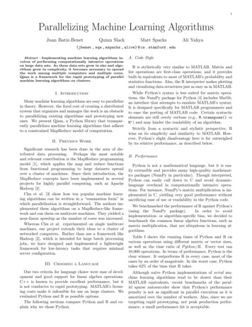
Numax RA, FroMax RA and NILE-Pro RA’s performance of producing linear, lowdimensional embeddings on this data set.Figure 7.2 plots the variation of the number of measurements M as a function ofthe isometry constant δ. We observe that NILE-Pro RA achieves the desired isometryconstant on the secants using by far the fewest number of measurements. FroMax RAperforms better for small δ due to the correlation between δ and q, as we discussedbefore. Moreover, both Numax RA and Fromax RA greatly outperform PCA, apopular embedding technique in the literature.Fig. 7.1. Our synthetic training set consists of sixty 256-dimensional random generated translating disks and squares figure.Fig. 7.2. A comparison of the isometry constant δ with the number of measurements for PCA,Numax RA, FroMax RA and NILE-Pro RA’s performance of producing linear, low-dimensionalembeddings.190
δ0.40.20.1#Data952005009520050095200500NILE-ProRk Rk uMaxRk able 7.2Comparison of runtime performance for FroMax RA, NILE-Pro RA, and NuMax on subsetsof “5” images from MNIST.7.3. Runtime Performance on MNIST with Rank Adjustment. In thisexperiment, we consider a more challenging, real-world data set, the MNIST dataset, see figure 7.3. MNIST contains many digital images of handwritten digits andis a common benchmark data set for machine learning. We examine subsets of thetraining set for the digit “5”. We take subsets consisting of 95, 200, and 500 datapoints with original dimension 49.We test runtime performance of FroMax and NILE-Pro RA on these data sets.Our results may be found in Table 2.Fig. 7.3. Examples of 5 images from the MNIST dataset.Our experimental results show that NILE-Pro RA may perform significantly fasterand give a better optimal rank than NuMax while FroMax RA converges slower forlarger data sets. This may be due to the nature of the local minima found in FroMax;the estimate for P ΨT Ψ given for a larger rank does not correspond to the localminima for lower ranks so that this initialization is beneficial.Our results for FroMax RA reveal another issue with our rank adjustment method.FroMax RA appears to struggle with determining the optimal rank, sometimes perf
PRACTICAL ALGORITHMS FOR LEARNING NEAR-ISOMETRIC LINEAR EMBEDDINGS JERRY LUOy, KAYLA SHAPIROz, HAO-JUN MICHAEL SHIx, . University of California, Los Angeles, Los Angeles, CA 90024. (hjmshi@ucla.edu) . ear, near-isometric, or distance preserving, embedding such that Xcan be mapped to a subspace of dimension M O(logQ) with high probability. .